Meep Introduction
From AbInitio
(diff) ←Older revision | Current revision | Newer revision→ (diff)
| |
| Meep |
| Download |
| Release notes |
| FAQ |
| Meep manual |
| Introduction |
| Installation |
| Tutorial |
| Reference |
| C++ Tutorial |
| C++ Reference |
| Acknowledgements |
| License and Copyright |
Meep implements the finite-difference time-domain (FDTD) method for computational electromagnetism. This is a widely used technique in which space is divided into a discrete grid and then the fields are evolved in time using discrete time steps—as the grid and the time steps are made finer and finer, this becomes a closer and closer approximation for the true continuous equations, and one can simulate many practical problems essentially exactly.
In this section, we introduce the equations and the electromagnetic units employed by Meep, the FDTD method, and Meep's approach to FDTD. Also, FDTD is only one of several useful computational methods in electromagnetism, each of which has their own special uses—we mention a few of the other methods, and try to give some hints as to which applications FDTD is best suited for and when you should consider a different method.
Contents |
Maxwell's equations
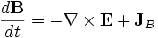
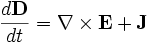
Meep simulates Maxwell's equations, which describe the interactions of electric (E) and magnetic (H) fields with one another and with matter and sources. In particular, the equations for the evolution of the fields are:
| 
|
| 
|
Where D is the displacement field, ε is the dielectric constant, J is the current density, and JB is the magnetic-charge current density. (Magnetic currents are a convenient computational fiction in some situations.) B is the magnetic flux density (often called the magnetic field), but currently μ (the magnetic permeability) is always 1 in Meep so we don't need to distinguish between B and H.
Most generally, ε depends not only on position but also on frequency (material dispersion) and on the field E itself (nonlinearity), and may include loss or gain. These effects are supported in Meep and are described in Dielectric materials in Meep.
Units in Meep
You may have noticed the lack of annoying constants like ε0, μ0, c, and 4π — that's because Meep uses "dimensionless" units where all these constants are unity (you can tell it was written by theorists). As a practical matter, almost everything you might want to compute (transmission spectra, frequencies, etcetera) is expressed as a ratio anyway, so the units end up cancelling.
In particular, because Maxwell's equations are scale invariant (multiplying the sizes of everything by 10 just divides the corresponding solution frequencies by 10), it is convenient in electromagnetic problems to choose scale-invariant units. That means that we pick some characteristic lengthscale in the system, a, and use that as our unit of distance.
Moreover, since c = 1 in Meep units, a is our unit of time as well. In particular, the frequency ω in Meep (corresponding to a time dependence exp( − iωt)) is always specified in units of 2πc / a, which is equivalent to specifying ω as 1 / T: the inverse of the optical period T in units of a / c. This, in turn is equivalent to specifying ω as a / λ where λ is the vacuum wavelength. (A similar scheme is used in MPB.)
For example, suppose we are describing some nanophotonic structure at infrared frequencies, where it is convenient to specify distances in microns. Thus, we let a = 1μm. Then, if we want to specify a source corresponding to λ = 1.55μm, we specify the frequency ω as 1/1.55 = 0.6452. If we want to run our simulation for 100 periods, we then run it for 155 time units (= 100 / ω).
A transmission spectrum, for example, would be a ratio of transmitted to incident intensities, so the units of E are irrelevant (unless there are nonlinearities).
Finite-difference time-domain methods
FDTD methods divide space and time into a finite rectangular grid. As described below, Meep tries to hide this discreteness from the user as much as possible, but there are a few consequences of discretization that it is good to be familiar with.
Perhaps the most important thing you need to know is this: if the grid has some spatial resolution Δx, then our discrete time-step Δt is given by Δt = CΔx, where C is the Courant factor and must satisfy 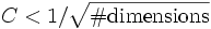 in order for the method to be stable (not diverge). (In Meep, C = 0.5 by default (which is sufficient for 1 to 3 dimensions), but can be changed by the user.) This means that when you double the grid resolution, the number of time steps doubles as well (for the same simulation period). Thus, in three dimensions, if you double the resolution, then the amount of memory increases by 8 and the amount of computational time increases by (at least) 16.
The second most important thing you should know is that, in order to discretize the equations with second-order accuracy, FDTD methods store different field components at different grid locations. This discretization is known as a Yee lattice, and is described in more detail at: Yee lattices. As a consequence, Meep must interpolate the field components to a common point whenever you want to combine, compare, or output the field components (e.g. in computing energy density or flux). Most of the time, you don't need to worry too much about this interpolation since it is automatic. However, because it is a simple linear interpolation, while E and D may be discontinuous across dielectric boundaries, it means that the interpolated E and D fields may be less accurate than you might expect right around dielectric interfaces.
Many references are available on FDTD methods for electromagnetism. See, for example:
- Allen Taflove and Susan C. Hagness, Computational Electrodynamics: The Finite-Difference Time-Domain Method (Artech: Norwood, MA, 2000).
The illusion of continuity in Meep
Although FDTD inherently uses discretized space and time, as much as possible Meep attempts to maintain the illusion that you are using continuous system. At the beginning of the simulation, you specify the spatial resolution, but from that point onwards you generally work in continuous coordinates in your chosen units (see units in Meep, above).
For example, you specify the dielectric function as a continuous function ε(x), or as a set of solid objects like spheres, cylinders, etcetera, and Meep is responsible for figuring out how they are to be represented on a discrete grid. Or if you want to specify a point source, you simply specify the point x where you want the source to reside—Meep will figure out the closest grid points to x and add currents to those points, weighted according to their distance from x. If you change x continously, the current in Meep will also change continuously (by changing the weights). If you ask for the flux through a certain rectangle, then Meep will linearly interpolate the field values from the grid onto that rectangle.
In general, the philosophy of the Meep interface is pervasive interpolation, so that if you change any input continously then the response of the Meep simulation will change continuously as well, and so that it will converge as rapidly and as smoothly as possible to the continuous solution as you increase the spatial resolution.
The one exception to this rule is in the dielectric function, where we are still determining the best method of sub-pixel averaging to map the continuous ε onto the discretized ε. Since this sub-pixel averaging is still somewhat experimental, it is currently turned off by default; it can be enabled with the enable-eps-averaging? input parameter (see the user reference). If the averaging is turned off, as you change the structure there will be a "stair-stepping" effect where the discretized ε changes in jumps as pixel boundaries are crossed.
