Meep Introduction

From AbInitio

Meep

Download

Release notes

FAQ

Meep manual

Introduction

Installation

Tutorial

Reference

C++ Tutorial

C++ Reference

Acknowledgements

License and Copyright

Meep implements the 'finite-difference time-domain (FDTD) method for computational electromagnetism. This is a widely used technique in which space is divided into a discrete grid and then the fields are evolved in time using discrete time steps—as the grid and the time steps are made finer and finer, this becomes a closer and closer approximation for the true continuous equations, and one can simulate many practical problems essentially exactly.

In this section, we introduce the equations and the electromagnetic units employed by Meep, the FDTD method, and Meep's approach to FDTD. Also, FDTD is only one of several useful computational methods in electromagnetism, each of which has their own special uses—we mention a few of the other methods, and try to give some hints as to which applications FDTD is best suited for and when you should consider a different method.

Contents 1 Maxwell's equations 1.1 Material dispersion and nonlinearity 1.1.1 Dispersion 1.1.2 Loss and gain 1.1.3 Nonlinearity 1.2 Units in Meep 2 Finite-difference time-domain methods 2.1 The illusion of continuity in Meep 3 Other computational methods 4 Applications of FDTD 4.1 Field patterns and Green's functions 4.2 Transmission/reflection spectra 4.3 Resonant modes

Maxwell's equations

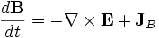
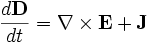
Meep simulates Maxwell's equations, which describe the interactions of electric (E) and magnetic (H) fields with one another and with matter and sources. In particular, the equations for the evolution of the fields are:

Where D is the displacement field, ε is the dielectric constant, J is the current density, and J_B is the magnetic-charge current density. (Magnetic currents are a convenient computational fiction in some situations.) B is the magnetic flux density (often called the magnetic field), but currently μ (the magnetic permeability) is always 1 in Meep so we don't need to distinguish between B and H.

You may have noticed the lack of annoying constants like ε₀, μ₀, c, and 4π — that's because Meep uses "dimensionless" units where all these constants are unity (you can tell it was written by theorists). As a practical matter, almost everything you might want to compute is expressed as a ratio anyway, so the units end up cancelling; see Units in Meep, below.

Material dispersion and nonlinearity

The material structure is determined by the dielectric function ε(x), but ε is not only a function of position — in general, it also depends on frequency (material dispersion) and on the electric field E itself (nonlinearity). Material dispersion, in turn, is generally associated with absorption loss in the material, or possibly gain. All of these effects can be simulated in Meep, with certain restrictions.

Dispersion

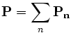
Physically, material dispersion arises because the polarization of the material does not respond instantaneously to an applied field E, and this is essentially the way that it is implemented in FDTD. In particular, is expanded to:

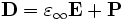
where is the instantaneous dielectric function (the infinite-frequency response) and P is the polarization density in the material. P, in turn, has its own time-evolution equation, and the exact form of this equation determines the frequency-dependence ε(ω). In particular, Meep supports any material dispersion of the form of a sum of harmonic resonances:

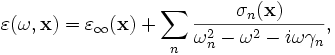
where ω_n and γ_n are user-specified constants and is a user-specified function of position. This corresponds to evolving P via the equations:

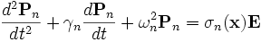
That is, we must store and evolve a set of auxiliary fields along with the electric field in order to keep track of the polarization P. Essentially any ε(ω) could be modeled by including enough of these polarization fields — Meep allows you to specify any number of these, limited only by computer memory and time (which must increase with the number of polarization terms you require).

Loss and gain

If γ above is nonzero, then the dielectric function ε(ω) becomes complex, where the imaginary part is associated with absorption loss in the material if it is positive, or gain if it is negative.

If you look at Maxwell's equations, then plays exactly the same role as a current . Just as is the rate of change of mechanical energy (the power expended by the electric field on moving the currents), the rate at which energy is lost to absorption is given by:

absorption rate

Meep can keep track of this energy, which for gain gives the amount of energy expended in amplifying the field. Using this energy, Meep supports the idea of a saturable gain (e.g. a situation in which there is a depletable population inversion causing the gain). For more information, see saturable gain in Meep.

Nonlinearity

In general, ε can be changed by the E field itself, with:

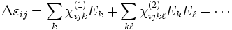
where the ij is the index of the change in the 3×3 ε tensor and the χ terms are the nonlinear susceptibilities. The χ⁽¹⁾ term is the Pockels effect and the χ⁽²⁾ term is the Kerr effect. (The above expansion assumes that the nonlinearity is instantaneous; more generally, Δε would depend on some average of the fields at previous times.)

Currently, Meep supports instantaneous, isotropic Kerr nonlinearities, where Failed to parse (unknown error): \chi_{ijk\ell}^{(2)} = \chi^{{2)} \cdot \delta_{ij} \delta{k\ell} , so that

Failed to parse (unknown error): \Delta\varepsilon = \chi^{{2)} |\mathbf{E}|^2 .

Units in Meep

Finite-difference time-domain methods

The illusion of continuity in Meep

Although FDTD inherently uses discretized space and time, as much as possible Meep attempts to maintain the illusion that you are using continuous system.

Other computational methods

Applications of FDTD

Field patterns and Green's functions

Transmission/reflection spectra

Resonant modes