Meep Introduction
From AbInitio
| Revision as of 06:16, 22 October 2005 (edit) Stevenj (Talk | contribs) (→Units in Meep) ← Previous diff |
Revision as of 06:22, 22 October 2005 (edit) Stevenj (Talk | contribs) (→Units in Meep) Next diff → |
||
| Line 32: | Line 32: | ||
| For example, suppose we are describing some nanophotonic structure at infrared frequencies, where it is convenient to specify distances in microns. Thus, we let <math>a = 1 \mu\textrm{m}</math>. Then, if we want to specify a source corresponding to <math>\lambda = 1.55 \mu\textrm{m}</math>, we specify the frequency ω as 1/1.55 = 0.6452. If we want to run our simulation for 100 periods, we then run it for 155 time units (= 100 / ω). | For example, suppose we are describing some nanophotonic structure at infrared frequencies, where it is convenient to specify distances in microns. Thus, we let <math>a = 1 \mu\textrm{m}</math>. Then, if we want to specify a source corresponding to <math>\lambda = 1.55 \mu\textrm{m}</math>, we specify the frequency ω as 1/1.55 = 0.6452. If we want to run our simulation for 100 periods, we then run it for 155 time units (= 100 / ω). | ||
| - | A transmission spectrum, for example would be a ratio of transmitted to incident intensities, so the units of '''E''' are irrelevant (unless there are nonlinearities). | + | A transmission spectrum, for example, would be a ratio of transmitted to incident intensities, so the units of '''E''' are irrelevant (unless there are nonlinearities). |
| == Finite-difference time-domain methods == | == Finite-difference time-domain methods == | ||
Revision as of 06:22, 22 October 2005
| |
| Meep |
| Download |
| Release notes |
| FAQ |
| Meep manual |
| Introduction |
| Installation |
| Tutorial |
| Reference |
| C++ Tutorial |
| C++ Reference |
| Acknowledgements |
| License and Copyright |
Meep implements the 'finite-difference time-domain (FDTD) method for computational electromagnetism. This is a widely used technique in which space is divided into a discrete grid and then the fields are evolved in time using discrete time steps—as the grid and the time steps are made finer and finer, this becomes a closer and closer approximation for the true continuous equations, and one can simulate many practical problems essentially exactly.
In this section, we introduce the equations and the electromagnetic units employed by Meep, the FDTD method, and Meep's approach to FDTD. Also, FDTD is only one of several useful computational methods in electromagnetism, each of which has their own special uses—we mention a few of the other methods, and try to give some hints as to which applications FDTD is best suited for and when you should consider a different method.
Contents |
Maxwell's equations
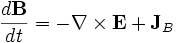
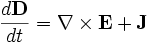
Meep simulates Maxwell's equations, which describe the interactions of electric (E) and magnetic (H) fields with one another and with matter and sources. In particular, the equations for the evolution of the fields are:
| 
|
| 
|
Where D is the displacement field, ε is the dielectric constant, J is the current density, and JB is the magnetic-charge current density. (Magnetic currents are a convenient computational fiction in some situations.) B is the magnetic flux density (often called the magnetic field), but currently μ (the magnetic permeability) is always 1 in Meep so we don't need to distinguish between B and H.
Most generally, ε depends not only on position but also on frequency (material dispersion) and on the field E itself (nonlinearity), and may include loss or gain. These effects are supported in Meep and are described in Dielectric materials in Meep.
Units in Meep
You may have noticed the lack of annoying constants like ε0, μ0, c, and 4π — that's because Meep uses "dimensionless" units where all these constants are unity (you can tell it was written by theorists). As a practical matter, almost everything you might want to compute (transmission spectra, frequencies, etcetera) is expressed as a ratio anyway, so the units end up cancelling.
In particular, because Maxwell's equations are scale invariant (multiplying the sizes of everything by 10 just divides the corresponding solution frequencies by 10), it is convenient in electromagnetic problems to choose scale-invariant units. That means that we pick some characteristic distance lengthscale in the system, a, and use that as our unit of distance.
Moreover, since c = 1 in Meep units, a is our unit of time as well. In particular, the frequency ω in Meep (corresponding to a time dependence exp( − iωt)) is always specified in units of 2πc / a, which is equivalent to specifying ω as the 1 / T (the inverse of the optical period T in units of a / c), which in turn is equivalent to specifying a / λ where λ is the vacuum wavelength.
For example, suppose we are describing some nanophotonic structure at infrared frequencies, where it is convenient to specify distances in microns. Thus, we let a = 1μm. Then, if we want to specify a source corresponding to λ = 1.55μm, we specify the frequency ω as 1/1.55 = 0.6452. If we want to run our simulation for 100 periods, we then run it for 155 time units (= 100 / ω).
A transmission spectrum, for example, would be a ratio of transmitted to incident intensities, so the units of E are irrelevant (unless there are nonlinearities).
Finite-difference time-domain methods
The illusion of continuity in Meep
Although FDTD inherently uses discretized space and time, as much as possible Meep attempts to maintain the illusion that you are using continuous system.
