Casimir calculations in Meep
From AbInitio
| Revision as of 17:45, 31 August 2009 (edit) Alexrod7 (Talk | contribs) (→Example: two-dimensional blocks) ← Previous diff |
Revision as of 18:00, 31 August 2009 (edit) Alexrod7 (Talk | contribs) Next diff → |
||
| Line 127: | Line 127: | ||
| ===Sources=== | ===Sources=== | ||
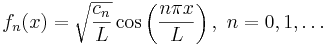
| - | ==Sources== | + | In this problem we use a cosine basis for the sources. For each side of <math>S</math> and each non-negative integer <math>n</math>, this defines a source distribution: |
| - | + | ||
| <math> f_n(x) = \sqrt{\frac{c_n}{L}} \cos \left(\frac{n\pi x}{L}\right), ~n = 0,1,\ldots </math> | <math> f_n(x) = \sqrt{\frac{c_n}{L}} \cos \left(\frac{n\pi x}{L}\right), ~n = 0,1,\ldots </math> | ||
| Line 136: | Line 135: | ||
| where <math>c_n = 1</math> if <math>n=0</math> and <math>c_n=2</math> otherwise, <math>L</math> is the side length (if each side has a different length, then the functions <math>f_n(x)</math> will differ for each side). An illustration of these functions for the system under consideration is shown on the right. | where <math>c_n = 1</math> if <math>n=0</math> and <math>c_n=2</math> otherwise, <math>L</math> is the side length (if each side has a different length, then the functions <math>f_n(x)</math> will differ for each side). An illustration of these functions for the system under consideration is shown on the right. | ||
| - | As shown in the figure, any set of basis functions will give the same force once every function is included. One can equally well compute the force using a basis where each <math>f_n</math> is a <math>\delta</math> function. However, one would require many different point sources to get an accurate answer, whereas the cosine basis above requires only a few values of <math>n</math> before the answer has converged to high accuracy (this is discussed further in Part II). | + | For the simulation, we must truncate the sum over <math>n</math> to some finite upper limit <code>n-max</code>. Typically, a value of 10 is sufficient to get results to within 1%: |
| - | For the present example, the functions <math>f_n(x)</math> are easily defined in the ctl file: | + | (define-param n-max 10) |
| - | (define (dct X n source-size) | + | ===Simulation Parameters=== |
| - | (let* | + | |
| - | ((X-start (vector3+ X (vector3-scale 0.5 face-size)))) | + | |
| - | (x (vector3-x X-start)) | + | |
| - | (y (vector3-y X-start)) | + | |
| - | (kx (/ (* n pi) L)) | + | |
| - | (ky (/ (* n pi) L))) | + | |
| - | (* (sqrt (/ (if (= n 0) 1 2) L)) (cos (* kx x)) (cos (* ky y)))) | + | |
| - | The reason for the shift from <code>X</code> to <code>X-start</code> is that the origin of the dct functions is the endpoint of the line segment, while the origin for a function <code> (amp-func ...)</code> is taken to be the center of the surface. Also, we are allowed to insert both <code>(cos (* kx x))</code> and <code>(cos (* ky y))</code>, even though the face is actually one-dimensional. This is because, if the surface has zero size in one direction, that coordinate will always be zero (since the coordinates are relative to the center of the face), so the <code>(cos ...)</code> term in that direction will always be 1. Writing things this way merely simplifies the Scheme code. | + | Computing the Casimir force involves running several independent Meep simulations for each set of parameters. These parameters are grouped into the following lists: |
| - | A simulation is run for each <math>n</math>, each side of <math>S</math>, indexed by the integer <code>side</code>, and each source polarization. The source itself has the form: | + | (define pol-list (list Ex Ey Ez Hx Hy Hz)) ;source polarizations |
| + | (define side-list (list 0 1 2 3)) ;each side of the square surface S | ||
| + | (define n-list (if (eq? n-max 0) (list 0) (interpolate (- n-max 1) 0 n-max))) ;number of terms in source sum | ||
| - | <math> J(\textbf{x},t) = f_n(\textbf{x}) \delta(t),~~x \in S </math> | + | For each value of n, side number, and polarization, we run a short meep simulation. |
| - | This is defined using the <code>custom-src</code> function: | ||
| - | (define (update-sources) | ||
| - | (change-sources! | ||
| - | (list (make source | ||
| - | (src (make custom-src | ||
| - | (src-func (lambda (t) (if (= t (* 1.5 dt)) (/ 1 dt) 0) | ||
| - | (is-integrated? false) (start-time (- infinity)) (end-time 1))) | ||
| - | (center (list-ref face-centers side)) (size (list-ref face-sizes side)) | ||
| - | (component current-pol) (amplitude 1) | ||
| - | (amp-func (lambda (X) (dct X n (list-ref face-sizes side))))))) | ||
| - | where <code>dt</code> is the unit of time-stepping given by <code>(meep-fields-dt-get fields)</code>. | ||
| To illustrate the field profiles, below we show four snapshots at different times for what we term <math>\Gamma^E_{yy;n=2}(\textbf{x},t)</math>, the <math>y</math>-component of the electric field response to a <math>y</math>-polarized current source with spatial dependence <math>f_2(x)</math> | To illustrate the field profiles, below we show four snapshots at different times for what we term <math>\Gamma^E_{yy;n=2}(\textbf{x},t)</math>, the <math>y</math>-component of the electric field response to a <math>y</math>-polarized current source with spatial dependence <math>f_2(x)</math> | ||
Revision as of 18:00, 31 August 2009
| |
| Meep |
| Download |
| Release notes |
| FAQ |
| Meep manual |
| Introduction |
| Installation |
| Tutorial |
| Reference |
| C++ Tutorial |
| C++ Reference |
| Acknowledgements |
| License and Copyright |
Contents |
Computing Casimir forces with Meep
It is possible to use the Meep time-domain simulation code in order to calculate Casimir forces (and related quantities), a quantum-mechanical force that can arise even between neutral bodies due to quantum vacuum fluctuations in the electromagnetic field, or equivalently as a result of geometry dependence in the quantum vacuum energy.
Calculating Casimir forces in a classical finite-difference time-domain (FDTD) Maxwell simulation like Meep is possible because of a new algorithm described in:
- Alejandro W. Rodriguez, Alexander P. McCauley, John D. Joannopoulos, and Steven G. Johnson, "Casimir forces in the time domain: I. Theory," arXiv preprint archive article arXiv:0904.0267 (April 2009).
- Alexander P. McCauley, Alejandro W. Rodriguez, John D. Joannopoulos, and Steven G. Johnson, "Casimir forces in the time domain: II. Applications," arXiv preprint archive article arXiv:0906.5170 (June 2009).
These papers describe how any time-domain code may be used to efficiently compute Casimir forces without modification of the internal code. The newest version of Meep contains several optimizations of these algorithms, allowing for very rapid computation of Casimir forces (reasonably-sized two-dimensional systems can be solved in a matter of seconds).
This page will provide some tutorial examples showing how these calculations are performed for simple geometries. For a derivation of these methods, the reader is referred to the papers above, which will be referred to as Part I and Part II in this webpage.
Introduction
In this section, we introduce the equations and basic considerations involved in computing the force using the method presented in Rodriguez et. al. (arXiv:0904.0267). Note that we keep the details of the derivation to a minimum and instead focus on the calculational aspects of the resulting algorithm.
The general setup for a Casimir force computation is shown in the following figure:


The goal is to determine the Casimir force on one object (shown in red) due to the presence of other objects (blue).
Classically, the force on red object due to the electromagnetic field can be computed by integrating the Maxwell stress tensor '''M'''ij(ref: Griffiths) over frequency and over any surface enclosing only that object, shown below:
The classical force is then:
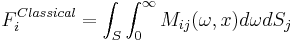
where the Maxwell stress tensor is given by:

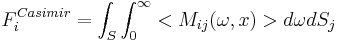
[ref] showed the the Casimir force can be obtained by a similar integral, except that the stress tensor is replaced with the expectation value of the corresponding operator in the quantum-mechanical grounds state of the system:
In Part I, it is shown how this formulation can be turned into an algorithm for computing Casimir forces in the time-domain. The reader is referred there for details. Below we present the basic steps used in our implementation.
Implementation
The basic steps involved in computing the Casimir force on an object are:
1. Surround the object for which the force is to be computed with a simple, closed surface S. It is often convenient to make S a rectangle in two dimensions or a rectangular prism in three dimensions. This is illustrated below:
In this calculation, we determine the force on the object (shown in red) due to the presence of other objects (blue).
2. Add a uniform, frequency-independent conductivity σ to the dielectric response of every object (which is easily done Meep). The purpose of this is to rapidly reduces the time required for the simulations below. As discussed in Part I, adding this conductivity in the right way leaves the result for the force unchanged.
3. Determine the Green's function along S. This is done by measureing the electric E and magnetic H fields on S in response to a set of different current distributions on S (more on the form of these currents later).
4. Integrate these fields over the enclosing surface S at each time step, and then integrate this result, multiplied by a known function g( − t), over time t.
The Casimir force is given by an expression of the form:
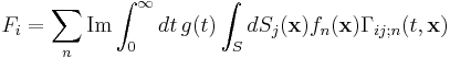
where the Γij;n are the fields in response to sources related to the functions fn (discussed in detail later), S is an arbitrary closed surface enclosing the object for which we want to compute the Casimir force, g(t) is a known function, and the index n ranges over all of the integers.
The functions  are related to the Maxwell stress tensor introduced in the previous section. Here the frequency integration has been turned into an integration over time, which is especially suited for our purposes.
Note that the precise implementation of step (3)
will greatly affect the efficiency of the method. For example,
computing the fields due to each source at each point on the surface
separately requires a separate Meep calculation for each source (and
polarization). This corresponds to taking 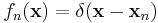 for each point
  , and the sum over n becomes an integration over S. As described in Part II (arXiv:0906.5170), we are free to take fn to be any basis of orthogonal functions. Picking an extended basis (e.g. cosine functions or complex exponentials eikx) greatly reduces the number of simulations required.
Example: two-dimensional blocks
In this section we calculate the Casimir force in the two-dimensional Casimir piston configuration (Rodriguez et. al, Physical Review Letters, vol 99, p 080401 2007) shown below:

This is described in the sample file rods-plates.ctl included in the examples directory. The dashed red lines indicate the surface S. This system consists of two metal  squares in between metallic sidewalls.
First define the geometry, consisting of the two metal sidewalls (each 2 pixels thick) and the two blocks:
 (define a 1)
 (define-param h 0.5)
 (set! geometry
    (list (make block (center 0 (+ (/ a 2) h (/ resolution))) ;upper sidewall
                                  (size infinity (/ 2 resolution) infinity) (material metal))
            (make block (center 0 (- (+ (/ a 2) h (/ resolution)))) ;lower sidewall
                                  (size infinity (/ 2 resolution) infinity) (material metal))
            (make block (center a 0) (size a a infinity) (material metal)) ;right block
            (make block (center (- a) 0) (size a a infinity) (material metal)))) ;left block
Define an air buffer on either side of the blocks and the PML thickness. Then set the computational cell size, and add in pml on the left/right sides:
 (define buffer 1)
 (define dpml 1)
 (set! geometry-lattice (make lattice (size (+ dpml buffer a a a buffer dpml) (+ (/ 2 resolution) h a h (/ 2 resolution)) no-size)))
 (set! pml-layers (list (make pml (thickness dpml) (direction X))))
Define the source surface S; here we take it to be a square with edges 0.05 away from the right block on each side:
(define S (volume (center a 0) (size (+ a 0.1) (+ a 0.1))))
As described in Part II, we add a uniform, frequency-independent D-conductivity σ everywhere:
(define Sigma 1)
(note that "sigma" is another built-in Meep parameter, so here we use a capital S).
As discussed in Part I, the optimal value of σ depends on the system under consideration. In our case, σ = 1 is optimal or nearly optimal. With this choice value of Sigma<\code>, we can use a very short runtime <code>T for the simulation:
(define-param T 20)
The only thing left to define is the function g( − t). This is done with the Meep function (make-casimir-g T dt Sigma ft):
(define gt (make-casimir-g T (/ Courant resolution) Sigma Ex))
Here we can pass in either field type Ex or Hx. Since the E/H fields are defined for integer/half-integer units of the time step dt, we technically require a different g(t) for both polarizations, and this option is allowed. However, for this example we get sufficient accuracy by using the same function for all polarizations.
Sources
In this problem we use a cosine basis for the sources. For each side of S and each non-negative integer n, this defines a source distribution:

where cn = 1 if n = 0 and cn = 2 otherwise, L is the side length (if each side has a different length, then the functions fn(x) will differ for each side). An illustration of these functions for the system under consideration is shown on the right.
For the simulation, we must truncate the sum over n to some finite upper limit n-max. Typically, a value of 10 is sufficient to get results to within 1%:
(define-param n-max 10)
Simulation Parameters
Computing the Casimir force involves running several independent Meep simulations for each set of parameters. These parameters are grouped into the following lists:
 (define pol-list (list Ex Ey Ez Hx Hy Hz))          ;source polarizations
 (define side-list (list 0 1 2 3))                            ;each side of the square surface S
 (define n-list (if (eq? n-max 0) (list 0) (interpolate (- n-max 1) 0 n-max)))    ;number of terms in source sum
For each value of n, side number, and polarization, we run a short meep simulation.
To illustrate the field profiles, below we show four snapshots at different times for what we term 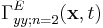 , the y-component of the electric field response to a y-polarized current source with spatial dependence f2(x)

At each time-step, the fields are integrated over S, weighted by both fn(x) and g(t), yielding a differential increment in the force as a function of time:
![dF_{n} = \mathrm{Im}[g(t)] \int_S dS_j(\textbf{x}) f_n(\textbf{x}) \Gamma_{ij;n}(t,\textbf{x})](/wiki/images/math/a/4/b/a4bc1a92d75e083b25c5251163c7d0a6.png)
Computation of g(t)
As discussed in Part I, the function g(t) is directly computed as the Fourier transform of a function of real frequency ξ, g(ξ). This function is given by:
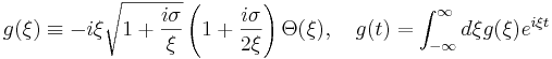
This Fourier transform can be computed numerically. However, as discussed in Part II, g(ξ) diverges in both the low-ξ and high-ξ limits, making numerical computation of the transform cumbersome. A method around this issue (discussed in the appendix of Part II) is to subtract off these asymptotic terms and evaluate their Fourier transforms analytically. The remaining function is bounded for all frequency and is easily handled numerically.
A Fourier transform is still clumsy to implement directly through the Scheme front-end. This is why, in the newest release of Meep, we have included a function (make-casimir-g ...) which will return a list whose values are g(t) where t is given in increments of the time-domain simulation dt:
(define gt (make-casimir-g T dt Sigma [eps-omega] [Tfft]))
Here T is the total simulation time, and the optional argument eps-omega accounts for dispersive materials (the influence of dispersion is discussed in Part I) and Tfft controls the frequency resolution of the Fourier transform (dξ˜1 / TFFT). By default, eps-omega is NULL and Tfft equals 10T. For many cases, however, T < 50 is often sufficient to obtain high convergence. In this case, a value of Tfft on the order of 103 or greater is recommended.
Integration of the fields
As with the construction of g(t), the integration of the fields along S, weighted by the function fn(x), can be done in any version of meep through the Scheme interface. However, in this form, every pixel communicates through the Scheme interpreter at every timestep. This significantly slows down computation time; in fact, in two dimensions it dominates the actual time-stepping for resolutions below 400!
To circumvent this, the newest version of meep also has a built-in field-integration routine, (meep-fields-casimir-stress-dct-integral ...), which will automatically integrate the field response Γij;n along a specified face of S. This value is then added to the current force in direction x.
We compress both of these steps into one function, (integrate-function), which will be called at every time step:
(define counter 0)
 (define (integrate-function)
     (set! Gamma-integral-X
        (meep-fields-casimir-stress-dct-integral fields X current-dir n n 0 E-stuff current-face))
     (set! Force-x
        (+ Force-x (* dt
                     (imag-part (list-ref gt counter))
                     current-orientation
                     Gamma-integral-X))
    (set! counter (+ counter 1)))
Now define a procedure for running a simulation for each side of S for each electric field polarization curr-pol:
 (define (run-one-simulation curr-pol)
   (begin
       (set! current-pol curr-pol)
       (do ((i 0 (1+ i))) ((= i (length face-centers))) ;Faces of S
          (begin
             (update-sources)
             (set! current-face (volume (center (list-ref face-centers i)) (size (list-ref face-sizes i))))
             (run-until Tmax integrate function)
             (restart-fields) (set! counter 0)))))
The appropriate run time T depends upon the system under consideration. The the example of the double blocks, we find that by T = 40 the force has converged to within  of its final value.
Now we simply run one of these simulations for each polarization:
 (define pols-list (list Ex Ey Ez))
 (map run-one-simulation pols-list)
Magnetic field contribution
As discussed above, we must now run a separate set of simulations to get the contribution from magnetic sources. This is easily done in Meep by resetting the geometry so that  and μ are switched:
(reset-meep)
 (set! my-metal (make medium (epsilon 1) (mu -1e20) (D-conductivity Sigma))
 (set! default-material my-air)
 (set! geometry
       (list (make block (center   a   0) (size a a infinity) (material my-metal))
             (make block (center (- a) 0) (size a a infinity) (material my-metal))))
(map run-one-simulation pols-list)
Notice that we still use a D-conductivity, rather than a B-conductivity as one might expect; remember that this conductivity is introduced as a mathematical construction. The physical system has no dissipation, and the appropriate way to input the conductivity is in this form (this is discussed in Part I). Otherwise, the simulation proceeds exactly as before.
Results
The result, when sampled over many values of h, is a force curve that varies non monotonically in h:

Using the optimizations discussed above, it takes roughly 20 seconds to run simulation at resolution 40 for each value of n, including all sides of S and all field polarizations. Typically, only  are needed to get the force to high precision, so the Casimir force for this system can be determined in under two minutes on a single processor
Example: dispersive materials
[coming soon]
Example: cylindrical symmetry
[coming soon]
Example: three-dimensional computations
[coming soon]
