Casimir calculations in Meep

It is possible to use the Meep time-domain simulation code in order to calculate Casimir forces (and related quantities), a quantum-mechanical force that can arise even between neutral bodies due to quantum vacuum fluctuations in the electromagnetic field, or equivalently as a result of geometry dependence in the quantum vacuum energy.

Calculating Casimir forces in a classical time-domain Maxwell simulation like Meep is possible because of a new algorithm described in:

Alejandro W. Rodriguez, Alexander P. McCauley, John D. Joannopoulos, and Steven G. Johnson, "Casimir forces in the time domain: I. Theory," arXiv preprint archive article arXiv:0904.0267 (April 2009).
Alexander P. McCauley, Alejandro W. Rodriguez, John D. Joannopoulos, and Steven G. Johnson, "Casimir forces in the time domain: II. Applications," arXiv preprint archive article arXiv:0906.5170 (June 2009).

This page will provide some tutorial examples showing how these calculations are performed for simple geometries.

Introduction

In this section, we introduce the equations and basic considerations involved in computing the force using the method presented in Rodriguez et. al. (arXiv:0904.0267). Note that we keep the details of the derivation to a minimum and instead focus on the calculational aspects of the resulting algorithm.

The basic steps involved in computing the Casimir force are:

1. Surround the object for which the force is to be computed with a simple, closed surface $S$ . It is often convenient to make $S$ a rectangle in two dimensions and a rectangular prism in three dimensions.

2. Add a uniform, frequency-independent conductivity $σ$ to the dielectric response of every object (which is easily done Meep). The purpose of this is to rapidly reduces the time required for the simulations below.

3. Measure the electric E and magnetic H fields on $S$ in response to a set of different current distributions on $S$ (more on the specific form of these currents later).

4. Integrate these fields over the enclosing surface $S$ at each time step, and then integrate this result, multiplied by a known function $g ( - t)$ , over time $t$ .

<ref>Note that the precise implementation of step (3) will greatly affect the efficiency of the method. For example, computing the fields due to each source at each point on the surface separately requires a separate Meep calculation for each source (and polarization). As described in <ref name="Rodriguez"/>, and further below, it is possible to modify these steps in order to optimize the calculation of the stress tensor over the spatial surface. For the purpose of this introduction, however, we do not require specific details on how we handle the spatial integration.</ref>

Example: two-dimensional blocks

In this section we calculate the Casimir force in the two-dimensional double-block configuration (Rodriguez et. al, Physical Review Letters, vol 99, p 080401 2007) shown below:

The dashed red lines indicate the surface $S$ . This system consists of two metal squares in between metallic sidewalls. As described in Part II, the first step is to add a uniform, frequency-independent D-conductivity $σ$ to all the dielectrics:

(define my-metal (make material (epsilon -1e20) (D-conductivity Sigma)))

As described in Part II, the next step is to pick a basis of functions ${f n}$ on $S$ , indexed by $n$ , such that these form a complete and orthonormal basis for all real-valued functions on $S$ . Since $S$ consists of four distinct line segments, we take a real cosine basis:

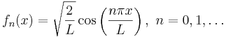
$f_n(x) = \sqrt{\frac{2}{L}} \cos \left(\frac{n\pi x}{L}\right), ~n = 0,1,\ldots$

where $L$ is the side length (if each side has a different length, then the functions $f n (x)$ will differ for each side).

Starting with $n = 0$ , an FDTD simulation is run with

The Casimir force on a body in the $i$ th direction is given by:

$F_i(t) = \textrm{Im} \, \frac{\hbar}{\pi} \sum_{n=0}^{T} g(-n\Delta t) \left[ \Gamma_i^E(n\Delta t) + \Gamma_i^H(n\Delta t) \right]$

where $Δ t$ denotes the temporal discretization inherent in any FDTD method (in meep, it is given by by $Δ t = S Δ x$ , as discussed in <ref>http://ab-initio.mit.edu/wiki/index.php/Meep_Introduction</ref>) and $T$ is a time cutoff which in the limit $T \to \infty$ yields the exact force (in the limit of infinite resolution $\Delta t \to 0$ ) and which can often be chosen to be small due to the exponential decay in the functions $Γ i$ . The Kernel $g ( - n Δ t)$ is given by a DFT of a pre-determined function:

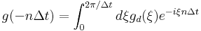
$g(-n \Delta t) = \int_{0}^{2\pi / \Delta t} d\xi g_d(\xi) e^{-i\xi n \Delta t}$

where,

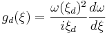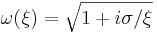$g_d(\xi) = \frac{\omega(\xi_d)^2}{i \xi_d} \frac{d\omega}{d\xi}$ , $\omega(\xi) = \sqrt{1 + i \sigma / \xi}$ and $\xi_d = \frac{2}{\Delta t} \sin \left(\frac{\xi \Delta t}{2}\right) e^{i \xi \Delta t / 2}$ .

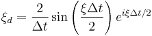Note that it is important to obtain $g ( - n Δ t)$ to good accuracy, but this is not a problem since the function need only be computed once for a given $σ$ and $Δ t$ . The $\Gamma_i^{E,H}$ are given by:

$\Gamma^E_i(n \Delta t) = \oint_{\vec{r} \in S} \sum_{j} \varepsilon(\vec{r}) \left[E_{i,j}(\vec{r},n \Delta t) - \frac{1}{2} \delta_{ij} E_{k,k}(\vec{r}, n \Delta t) \right]$

$\Gamma^H_i(n \Delta t) = \oint_{\vec{r} \in S} \sum_{j} \varepsilon(\vec{r}) \left[H_{i,j}(\vec{r},n \Delta t) - \frac{1}{2} \delta_{ij} H_{k,k}(\vec{r}, n \Delta t) \right]$ ,

where $E_{i,j}(\vec{r},t)$ and $H_{i,j}(\vec{r},t)$ are the electric and magnetic responses due to current sources placed along the surface of the body $S$ , and can be obtained as the output of a Meep calculation in a system with conductivity $σ D$ and $σ H$ , respectively (see Meep Introduction for more details on the various choices for conductivity).

Computing $Γ$ (t)

The only quantity above that requires Meep are the $Γ i$ functions, which are determined by the spatial integration of the $\vec{E}$ - and $\vec{H}$ -field response to a dipole current source. There are two ways to obtain $Γ i$ , briefly explained below.

A. Each source separately:

To obtain $E_{i,j}(\vec{r}',n\Delta t)$ at some $\vec{r}' \in S$ , one simply places a dipole current source $\vec{J}(\vec{r},t) = \delta(\vec{r}-\vec{r}') \delta(t) \hat{\vec{e}}_j$ (in the $j$ th direction) and finds the electric $\vec{E}(\vec{r},t)$ response (at the same point $\vec{r}=\vec{r}'$ ) in the presence of an electric conductivity (a non-zero $σ D$ in Meep). This calculation is then repeated for all $\vec{r}' \in S$ and all three polarizations $\hat{\vec{e}}_j$ of $\vec{J}$ , and can be performed in parallel, since each source is independent from one another. The same holds for the calculation of $H i, j$ except that in this case one employs magnetic currents $\vec{J}^H$ and conductivities $σ H$ .

B. Multipole expansion:

Coming soon.

Note that the surface of integration $S$ need not have any particular shape. In practice (2d and 3d), we often implement a simple square box (cube) enclosing the body of interest, for which the normals $d S j$ are easy to define (except at the corners, where they become ambiguous to define---due to the finite discretization, this is not a big concern, as seen from the example to follow).

Parallel plates

Coming soon.

2D geometry: square within square

To do.

Retrieved from "http://ab-initio.mit.edu/wiki/index.php/Casimir_calculations_in_Meep"

Category: Meep

 The dashed red lines indicate the surface <math>S</math>.  This system consists of two metal squares in between metallic sidewalls.  As described in Part II, the first step is to add a uniform, frequency-independent D-conductivity <math>\sigma</math> to all the dielectrics:
+(define my-metal (make material (epsilon -1e20) (D-conductivity Sigma)))
 As described in Part II, the next step is to pick a basis of functions <math>\lbrace f_n\rbrace</math> on <math>S</math>, indexed by <math>n</math>, such that these form a complete and orthonormal basis for all real-valued functions on <math>S</math>.  Since <math>S</math> consists of four distinct line segments, we take a real cosine basis:

Casimir calculations in Meep

From AbInitio

Revision as of 00:18, 2 July 2009

Contents