NLopt Tutorial
From AbInitio
(Difference between revisions)
| Revision as of 22:10, 13 November 2008 (edit) Stevenj (Talk | contribs) ← Previous diff |
Revision as of 22:11, 13 November 2008 (edit) Stevenj (Talk | contribs) (→Example nonlinearly constrained problem) Next diff → |
||
| Line 2: | Line 2: | ||
| ==Example nonlinearly constrained problem== | ==Example nonlinearly constrained problem== | ||
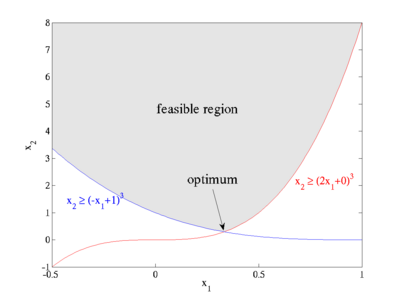
| - | + | [[Image:NLopt-example-constraints.png|right|thumb|400px|Feasible region for a simple example optimization problem with two nonlinear (cubic) constraints.]] | |
| As a first example, we'll look at the nonlinearly constrained minimization problem: | As a first example, we'll look at the nonlinearly constrained minimization problem: | ||
| Line 10: | Line 10: | ||
| for parameters ''a''<sub>1</sub>=2, ''b''<sub>1</sub>=0, ''a''<sub>2</sub>=-1, ''b''<sub>2</sub>=1. | for parameters ''a''<sub>1</sub>=2, ''b''<sub>1</sub>=0, ''a''<sub>2</sub>=-1, ''b''<sub>2</sub>=1. | ||
| - | [[Image:NLopt-example-constraints.png|right|thumb|400px|Feasible region for a simple example optimization problem with two nonlinear (cubic) constraints.]] | + | |
| The feasible region defined by these constraints is plotted at right: ''x''<sub>2</sub> is constrained to lie at the maximum of two cubics, and the optimum point is located at the intersection (1/3, 8/27) where the objective function takes on the value <math>\sqrt{8/27} \approx 0.5443310539518\ldots</math>. | The feasible region defined by these constraints is plotted at right: ''x''<sub>2</sub> is constrained to lie at the maximum of two cubics, and the optimum point is located at the intersection (1/3, 8/27) where the objective function takes on the value <math>\sqrt{8/27} \approx 0.5443310539518\ldots</math>. | ||
| (This problem is especially trivial, because by formulating it in terms of the cube root of ''x''<sub>2</sub> you can turn it into a linear-programming problem, but we won't do that here.) | (This problem is especially trivial, because by formulating it in terms of the cube root of ''x''<sub>2</sub> you can turn it into a linear-programming problem, but we won't do that here.) | ||
Revision as of 22:11, 13 November 2008
In this tutorial, we illustrate the usage of NLopt in various languages via one or two trivial examples.
Example nonlinearly constrained problem
As a first example, we'll look at the nonlinearly constrained minimization problem:

- subject to
 ,
,  , and
, and 
for parameters a1=2, b1=0, a2=-1, b2=1.
The feasible region defined by these constraints is plotted at right: x2 is constrained to lie at the maximum of two cubics, and the optimum point is located at the intersection (1/3, 8/27) where the objective function takes on the value  .
.
(This problem is especially trivial, because by formulating it in terms of the cube root of x2 you can turn it into a linear-programming problem, but we won't do that here.)

