NLopt Introduction

From AbInitio

NLopt

Download

Release notes

FAQ

NLopt manual

Introduction

Installation

Tutorial

Reference

Algorithms

License and Copyright

In this chapter of the manual, we begin by giving a general overview of the optimization problems that NLopt solves, the key distinctions between different types of optimization algorithms, and comment on ways to cast various problems in the form NLopt requires. We also describe the background and goals of NLopt.

Contents 1 Optimization problems 1.1 Global versus local optimization 1.2 Gradient-based versus derivative-free algorithms 1.3 Equivalent formulations of optimization problems 1.4 Equality constraints 2 Background and goals of NLopt

Optimization problems

NLopt addresses general nonlinear optimization problems of the form:

,

where f is the objective function and x represents the n optimization parameters. This problem may be subject to the bound contraints

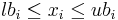for

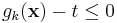
given lower bounds lb and upper bounds ub (which may be −∞ and/or +∞, respectively, for partially or totally unconstrained problems). One may also optionally have m nonlinear inequality constraints (sometimes called a nonlinear programming problem):

for .

A point x that satisfies all of the bound and inequality constraints is called a feasible point, and the set of all feasible points is the feasible region.

Note: in this introduction, we follow the usual mathematical convention of letting our indices begin with one. In the C programming language, however, NLopt follows C's zero-based conventions (e.g. i goes from 0 to m−1 for the constraints).

Global versus local optimization

NLopt includes algorithms to attempt either global or local optimization of the objective.

Global optimization is the problem of finding the feasible point x that minimizes the objective f(x) over the entire feasible region. In general, this can be a very difficult problem, becoming exponentially harder as the number n of parameters increases. In fact, unless special information about f is known, it is not even possible to be certain whether one has found the true global optimum, because there might be a sudden dip of f hidden somewhere in the parameter space you haven't looked at yet. However, NLopt includes several global optimization algorithms that work well on reasonably well-behaved problems, if the dimension n is not too large.

Local optimization is the much easier problem of finding a feasible point x that is only a local minimum: f(x) is less than or equal to the value of f for all nearby feasible points (the intersection of the feasible region with at least some small neighborhood of x). In general, a nonlinear optimization problem may have many local minima, and which one is located by an algorithm typically depends upon the starting point that the user supplies to the algorithm. Local optimization algorithms, on the other hand, can often quickly locate a local minimum even in very high-dimensional problems (especially using gradient-based algorithms).

There is a special class of convex optimization problems, for which both the objective and constraint functions are convex, where there is only one local minimum, so that a local optimization method find the global optimum. Typically, convex problems arise from functions of special analytical forms, such as linear programming problems, semidefinite programming, quadratic programming, and so on, and specialized techniques are available to solve these problems very efficiently. NLopt includes only general methods that do not assume convexity; if you have a convex problem you may be better off with a different software package, such as the CVX package from Stanford.

Gradient-based versus derivative-free algorithms

Especially for local optimization, the most efficient algorithms typically require the user to supply the gradient ∇f in addition to the value f(x) for any given point x. This exploits the fact that, in principle, the gradient can almost always be computed at the same time as the value of f using very little additional computational effort (at worst, about the same as that of evaluating f a second time). If the derivative of f is not obvious (e.g. if one has a simple analytical formula for f), one typically finds ∇f using an adjoint method, or possibly using automatic differentiation tools. Gradient-based methods are critical for the efficient optimization of very high-dimensional parameter spaces (e.g. n in the thousands or more).

On the other hand, computing the gradient is sometimes cumbersome and inconvenient if the objective function is supplied as a complicated program. It may even be impossible, if f is not differentiable (or worse, discontinuous). In such cases, it is often easier to use a derivative-free algorithm for optimization, which only requires that the user supply the function values f(x) for any given point x. Such methods typically must evaluate f for at least several-times-n points, however, so they are best used when n is small to moderate (up to hundreds).

NLopt provides both derivative-free and gradient-based algorithms with a common interface.

Note: If you find yourself computing the gradient by a finite-difference approximation (e.g. in one dimension), then you should use a derivative-free algorithm instead. Finite-difference approximations are not only expensive (2n function evaluations for the gradient using center differences), but they are also notoriously susceptible to roundoff errors unless you are very careful. On the other hand, finite-difference approximations are very useful to check that your analytical gradient computation is correct—this is always a good idea, because in my experience it is very easy to have bugs in your gradient code, and an incorrect gradient will cause weird problems with a gradient-based optimization algorithm.

Equivalent formulations of optimization problems

There are many equivalent ways to formulate a given optimization problem, even within the framework defined above, and finding the best formulation is something of an art.

To begin with a trivial example, suppose that you want to maximize the function g(x). This is equivalent to minimizing the function f(x)=−g(x). Because of this, there is no need for NLopt to provide separate maximization routines in addition to its minimization routines—the user can just flip the sign to do maximization.

A more interesting example is that of a minimax optimization problem, where the objective function f(x) is the maximum of N functions:

You could, of course, pass this objective function directly to NLopt, but there is a problem: it is not differentiable. Not only does this mean that the most efficient gradient-based algorithms are inapplicable, but even the derivative-free algorithms may be slowed down considerably. Instead, it is possible to formulate the same problem as a differentiable problem by adding a dummy variable t and N new nonlinear constraints (in addition to any other constraints):

subject to for .

This solves exactly the same minimax problem, but now we have a differentiable objective and constraints, assuming that the functions g_k are individually differentiable. Notice that, in this case, the objective function by itself is the boring linear function t, and all of the interesting stuff is in the constraints. This is typical of nonlinear programming problems.

Equality constraints

Suppose that you have one or more nonlinear equality constraints

.

In principle, each equality constraint can be expressed by two inequality constraints and , so you might think that any code that can handle inequality constraints can automatically handle equality constraints. In practice, this is not true—if you try to express an equality constraint as a pair of nonlinear inequality constraints, most algorithms will fail to converge.

Equality constraints typically require special handling because they reduce the dimensionality of the feasible region, and not just its size as for an inequality constraint. NLopt does not have code to handle nonlinear equality constraints.

Sometimes, it is possible to handle equality constraints by an elimination procedure: you use the equality constraint to explicitly solve for some parameters in terms of other unknown parameters, and then only pass the latter as optimization parameters to NLopt.

For example, suppose that you have a linear equality constraint:

for some constant matrix A. Given a particular solution ξ of these equations and a matrix N whose columns are a basis for the nullspace of A, one can express all possible solutions of these linear equations in the form:

for unknown vectors z. You could then pass z as the optimization parameters to NLopt, rather than x, and thus eliminate the equality constraint.

Background and goals of NLopt