Materials in Meep
From AbInitio
(diff) ←Older revision | Current revision | Newer revision→ (diff)
| |
| Meep |
| Download |
| Release notes |
| FAQ |
| Meep manual |
| Introduction |
| Installation |
| Tutorial |
| Reference |
| C++ Tutorial |
| C++ Reference |
| Acknowledgements |
| License and Copyright |
The material structure in Maxwell's equations is determined by the relative permittivity ε(x) and the relative permeability μ(x).
However, ε is not only a function of position. In general, it also depends on frequency (material dispersion) and on the electric field E itself (nonlinearity). It may also depend on the orientation of the field (anisotropy). Material dispersion, in turn, is generally associated with absorption loss in the material, or possibly gain. All of these effects can be simulated in Meep, with certain restrictions.
Similarly for the relative permeability μ(x), for which dispersion, nonlinearity, and anisotropy are all supported as well.
In this section, we describe the form of the equations and material properties that Meep can simulate. The actual interface with which you specify these properties is described in the Meep reference.
Contents |
Material dispersion
Physically, material dispersion arises because the polarization of the material does not respond instantaneously to an applied field E, and this is essentially the way that it is implemented in FDTD. In particular,  is expanded to:
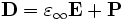
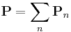
where  (which must be positive) is the instantaneous dielectric function (the infinite-frequency response) and P is the remaining frequency-dependent polarization density in the material. P, in turn, has its own time-evolution equation, and the exact form of this equation determines the frequency-dependence ε(ω). [Note that Meep's definition of ω uses a sign convention exp( − iωt) for the time dependence—ε formulas in engineering papers that use the opposite sign convention for ω will have a sign flip in all the imaginary terms below. If you are using parameters from the literature, you should use *positive* values of γ and σ as-is for loss; don't be confused by the difference in ω sign convention and flip the sign of the parameters.] In particular, Meep supports any material dispersion of the form of a sum of harmonic resonances, plus a term from the frequency-independent electric conductivity:
![\varepsilon(\omega,\mathbf{x}) = \left( 1 + \frac{i \cdot \sigma_D(\mathbf{x})}{\omega} \right) \left[ \varepsilon_\infty(\mathbf{x}) + \sum_n \frac{\sigma_n(\mathbf{x}) \cdot \omega_n^2 }{\omega_n^2 - \omega^2 - i\omega\gamma_n} \right] ,](/wiki/images/math/8/f/c/8fc5c3462c0242b22052fda9f2740504.png)
![= \left( 1 + \frac{i \cdot \sigma_D(\mathbf{x})}{2\pi f} \right) \left[ \varepsilon_\infty(\mathbf{x}) + \sum_n \frac{\sigma_n(\mathbf{x}) \cdot f_n^2 }{f_n^2 - f^2 - if\gamma_n/2\pi} \right] ,](/wiki/images/math/7/0/a/70a9538debac0832b4cc229e0fb5daef.png)
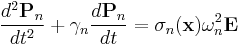
where σD is the electric conductivity, ωn and γn are user-specified constants (or actually, the numbers that one specifies are fn = ωn / 2π and γn / 2π), and the  is a user-specified function of position giving the strength of the n-th resonance. The σ parameters can be anisotropic (real-symmetric) tensors, while the frequency-independent term can be an arbitrary real-symmetric tensor as well. This corresponds to evolving P via the equations:
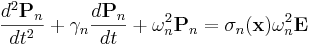
That is, we must store and evolve a set of auxiliary fields  along with the electric field in order to keep track of the polarization P. Essentially any ε(ω) could be modeled by including enough of these polarization fields — Meep allows you to specify any number of these, limited only by computer memory and time (which must increase with the number of polarization terms you require).
Note that the conductivity σD corresponds to an imaginary part of ε given by (not including the harmonic-resonance terms)  . When you specify frequency in Meep units, however, you are specifying f without the 2π, so the imaginary part of ε is
 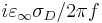 .
.
Meep also supports polarizations of the Drude form, typically used for metals:
which corresponds to a term of the following form in ε's ∑n:
 ,
,
which is equivalent to the Lorentzian model except that the  term has been omitted from the denominator, and asymptotes to a conductivity
  as
as  . In this case, is just a dimensional scale factor and has no interpretation as a resonance frequency.
Numerical stability
If you specify a Lorentzian resonance ωn at too high a frequency relative to the time discretization Δt, the simulation becomes unstable. Essentially, the problem is that you are trying to model a that oscillates too fast compared with the time discretization for the discretization to work properly. If this happens, you have three options: increase the resolution (which increases the resolution in both space and time), decrease the Courant factor (which decreases Δt compared to Δx), or use a different model function for your dielectric response.
Roughly speaking, the equation becomes unstable for ωnΔt / 2 > 1. (Note that, in Meep frequency units, you specify fn = ωn / 2π, so this quantity should be less than 1 / πΔt.) Meep will check a necessary stability criterion automatically and halt with an error message if it is violated.
Loss and gain
If γ above is nonzero, then the dielectric function ε(ω) becomes complex, where the imaginary part is associated with absorption loss in the material if it is positive, or gain if it is negative. Alternatively, a dissipation loss or gain may be added by a positive or negative conductivity, respectively—this is often convenient if you only care about the imaginary part of ε in a narrow bandwidth, and is described in detail below.
If you look at Maxwell's equations, then  plays exactly the same role as a current
  . Just as
  is the rate of change of mechanical energy (the power expended by the electric field on moving the currents), therefore, the rate at which energy is lost to absorption for is given by:
- absorption rate

Meep can keep track of this energy for the Lorentzian polarizability terms (but not for the conductivity terms), which for gain gives the amount of energy expended in amplifying the field. (This feature may be removed in a future Meep version.)
Conductivity and complex ε
Often, you only care about the absorption loss in a narrow bandwidth, where you just want to set the imaginary part of ε (or μ) to some known experimental value, in the same way that you often just care about setting a dispersionless real ε that is the correct value in your bandwidth of interest.
One approach to this problem would be allowing you to specify a constant (frequency-independent) imaginary part of ε, but this has the disadvantage of requiring the simulation to employ complex fields (doubling the memory and time requirements), and also tends to be numerically unstable. Instead, the approach in Meep is for you to set the conductivity σD (or σB for an imaginary part of μ), chosen so that 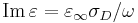 is the correct value at your frequency ω of interest. (Note that, in Meep, you specify f = ω / 2π instead of ω for the frequency, however, so you need to include the factor of 2π when computing the corresponding imaginary part of ε!) Conductivities can be implemented with purely real fields, so they are not nearly as expensive as implementing a frequency-independent complex ε or μ.
For example, suppose you want to simulate a medium with 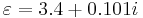 at a frequency 0.42 (in your Meep units), and you only care about the material in a narrow bandwidth around this frequency (i.e. you don't need to simulate the full experimental frequency-dependent permittivity). Then, in Meep, you could use
 (make medium (epsilon 3.4) (D-conductivity (/ (* 2 pi 0.42 0.101) 3.4)); i.e. 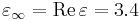 and
and  .
.
Note: the "conductivity" in Meep is slightly different from the conductivity you might find in a textbook, because (for computational convenience) it appears as  in our Maxwell equations rather than the more-conventional
  ; this just means that our definition is different from the usual electric conductivity by a factor of ε. Also, just as Meep uses the dimensionless relative permittivity for ε, it uses nondimensionalized units of 1/a (where a is your unit of distance) for the conductivities σD,B. If you have the electric conductivity σ in SI units and want to convert to σD in Meep units, you can simply use the formula:
 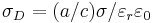 (where a is your unit of distance in meters, c is the vacuum speed of light in m/s,
  is the SI vacuum permittivity, and
  is the real relative permittivity).
Nonlinearity
In general, ε can be changed anisotropically by the E field itself, with:
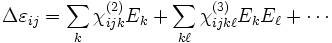
where the ij is the index of the change in the 3×3 ε tensor and the χ terms are the nonlinear susceptibilities. The χ(2) sum is the Pockels effect and the χ(3) sum is the Kerr effect. (If the above expansion is frequency-independent, then the nonlinearity is instantaneous; more generally, Δε would depend on some average of the fields at previous times.)
Currently, Meep supports instantaneous, isotropic Pockels and Kerr nonlinearities, corresponding to a frequency-independent 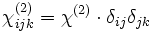 and
and 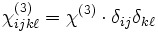 , respectively. Thus,

Here, "diag(E)" indicates the diagonal 3×3 matrix with the components of E along the diagonal.
Normally, for nonlinear systems you will want to use real fields E. (This is usually the default. However, Meep uses complex fields if you have Bloch-periodic boundary conditions with a non-zero Bloch wavevector k, or in cylindrical coordinates with  . In the C++ interface, real fields must be explicitly specified.)
For complex fields in nonlinear systems, the physical interpretration of the above equations is unclear because one cannot simply obtain the physical solution by taking the real part any more. In particular, Meep simply defines the meaning of the nonlinearity for complex fields as follows: the real and imaginary parts of the fields do not interact nonlinearly. That is, the above equation should be taken to hold for the real and imaginary parts (of E and D) separately. (e.g. |E|2 is the squared magnitude of the real part of E for when computing the real part of D, and conversely for the imaginary part.)
- Note: The behavior for complex fields was changed for Meep 0.10. Also, in Meep 0.9 there was a bug: when you specified χ(3) in the interface, you were actually specifying
 . This was fixed in Meep 0.10.
For a discussion of how to relate χ(3) in Meep to experimental Kerr coefficients, see Units and nonlinearity in Meep.
Magnetic permeability μ
All of the above features that are supported for the electric permittivity ε are also supported for the magnetic permeability μ. That is, Meep supports μ with dispersion from (magnetic) conductivity and Lorentzian resonances, as well as magnetic χ(2) and χ(3) nonlinearities. The description of these is exactly the same as above, so we won't repeat it here — just take the above descriptions and replace ε, E, D, and σD by μ, H, B, and σB, respectively.
