MPB User Reference
From AbInitio
(diff) ←Older revision | Current revision | Newer revision→ (diff)
| |
| MIT Photonic Bands |
| Download |
| Release notes |
| MPB manual |
| Introduction |
| Installation |
| User Tutorial |
| Data Analysis Tutorial |
| User Reference |
| Developer Information |
| Acknowledgements |
| License and Copyright |
Here, we document the features exposed to the user by the MIT Photonic-Bands package. We do not document the Scheme language or the functions provided by libctl (see also the libctl User Reference] section of the libctl Manual).
Contents |
Input Variables
These are global variables that you can set to control various parameters of the Photonic-Bands computation. They are also listed (along with their current values) by the (help) command. In brackets after each variable is the type of value that it should hold. (The classes, complex datatypes like geometric-object, are described in a later subsection. The basic datatypes, like integer, boolean, cnumber, and vector3, are defined by libctl.)
-
geometry[list ofgeometric-objectclass] - Specifies the geometric objects making up the structure being simulated. When objects overlap, later objects in the list take precedence. Defaults to no objects (empty list).
-
default-material[material-typeclass] - Holds the default material that is used for points not in any object of the geometry list. Defaults to air (epsilon of 1). See also
epsilon-input-file, below. -
ensure-periodicity[boolean] - If true (the default), then geometric objects are treated as if they were shifted by all possible lattice vectors; i.e. they are made periodic in the lattice.
-
geometry-lattice[latticeclass] - Specifies the basis vectors and lattice size of the computational cell (which is centered on the origin of the coordinate system). These vectors form the basis for all other 3-vectors in the geometry, and the lattice size determines the size of the primitive cell. If any dimension of the lattice size is the special value
no-size, then the dimension of the lattice is reduced (i.e. it becomes two- or one-dimensional). (That is, the dielectric function becomes two-dimensional; it is still, in principle, a three dimensional system, and the k-point vectors can be three-dimensional.) Generally, you should make anyno-sizedimension(s) perpendicular to the others. Defaults to the orthogonal x-y-z vectors of unit length (i.e. a square/cubic lattice). -
resolution[numberorvector3] - Specifies the computational grid resolution, in pixels per lattice unit (a lattice unit is one basis vector in a given direction). If
resolutionis avector3, then specifies a different resolution for each direction; otherwise the resolution is uniform. (The grid size is then the product of the lattice size and the resolution, rounded up to the next positive integer.) Defaults to10. -
grid-size[vector3] - Specifies the size of the discrete computational grid along each of the lattice directions. Deprecated: the preferred method is to use the
resolutionvariable, above, in which case thegrid-sizedefaults tofalse. To get the grid size you should instead use the(get-grid-size)function. -
mesh-size[integer] - At each grid point, the dielectric constant is averaged over a "mesh" of points to find an effective dielectric tensor. This mesh is a grid with
mesh-sizepoints on a side. Defaults to 3. Increasingmesh-sizemakes the the average dielectric constant sensitive to smaller structural variations without increasing the grid size, but also means that computing the dielectric function will take longer. (Using amesh-sizeof1turns off dielectric function averaging and the creation of an effective dielectric tensor at interfaces. Be sure you know what you're doing before you worsen convergence in this way.) -
dimensions[integer] - Explicitly specifies the dimensionality of the simulation; if the value is less than 3, the sizes of the extra dimensions in
grid-sizeare ignored (assumed to be one). Defaults to 3. Deprecated: the preferred method is to setgeometry-latticeto have size no-size in any unwanted dimensions. -
k-points[list ofvector3] - List of Bloch wavevectors to compute the bands at, expressed in the basis of the reciprocal lattice vectors. The reciprocal lattice vectors are defined as follows: Given the lattice vectors
Ri(not the basis vectors), the reciprocal lattice vectorGjsatisfiesRi * Gj = 2*Pi*deltai,j, wheredeltai,jis the Kronecker delta (1 fori = jand 0 otherwise). (Rifor anyno-sizedimensions is taken to be the corresponding basis vector.) Normally, the wavevectors should be in the first Brillouin zone ([#first-brillouin-zone see below]).k-pointsdefaults to none (empty list). -
num-bands[integer] - Number of bands (eigenvectors) to compute at each k point. Defaults to 1.
-
target-freq[number] - If zero, the lowest-frequency
num-bandsstates are solved for at each k point (ordinary eigenproblem). If non-zero, solve for thenum-bandsstates whose frequencies are have the smallest absolute difference withtarget-freq(special, "targeted" eigenproblem). Beware that the targeted solver converges more slowly than the ordinary eigensolver and may require a lowertoleranceto get reliable results. Defaults to 0. -
tolerance[number] - Specifies when convergence of the eigensolver is judged to have been reached (when the eigenvalues have a fractional change less than
tolerancebetween iterations). Defaults to 1.0e-7. -
filename-prefix[string] - A string prepended to all output filenames. Defaults to
""(no prefix). -
epsilon-input-file[string] - If this string is not
""(the default), then it should be the name of an HDF5 file whose first/only dataset defines a dielectric function (over some discrete grid). This dielectric function is then used in place ofdefault-material(i.e. where there are nogeometryobjects). The grid of the epsilon file dataset need not matchgrid-size; it is scaled and/or linearly interpolated as needed. The lattice vectors for the epsilon file are assumed to be the same asgeometry-lattice. [ Note that, even if the grid sizes match and there are no geometric objects, the dielectric function used by MPB will not be exactly the dielectric function of the epsilon file, unless you also setmesh-sizeto1(see above). ] -
eigensolver-block-size[integer] - The eigensolver uses a "block" algorithm, which means that it solves for several bands simultaneously at each k-point.
eigensolver-block-sizespecifies this number of bands to solve for at a time; if it is zero or >=num-bands, then all the bands are solved for at once. Ifeigensolver-block-sizeis a negative number, -n, then MPB will try to use nearly-equal block-sizes close to n. Making the block size a small number can reduce the memory requirements of MPB, but block sizes > 1 are usually more efficient (there is typically some optimum size for any given problem). Defaults to -11 (i.e. solve for around 11 bands at a time). -
simple-preconditioner?[boolean] - Whether or not to use a simplified preconditioner; defaults to
false(this is fastest most of the time). (Turning this on increases the number of iterations, but decreases the time for each iteration.) -
deterministic?[boolean] - Since the fields are initialized to random values at the start of each run, there are normally slight differences in the number of iterations, etcetera, between runs. Setting
deterministic?totruemakes things deterministic (the default isfalse). -
eigensolver-flags[integer] - This variable is undocumented and reserved for use by Jedi Masters only.
Predefined Variables
Variables predefined for your convenience and amusement.
-
air,vacuum[material-typeclass] - Two aliases for a predefined material type with a dielectric constant of 1.
-
nothing[material-typeclass] - A material that, effectively, punches a hole through other objects to the background (
default-materialorepsilon-input-file). -
infinity[number] - A big number (1.0e20) to use for "infinite" dimensions of objects.
Output Variables
Global variables whose values are set upon completion of the eigensolver.
-
freqs[list ofnumber] - A list of the frequencies of each band computed for the last k point. Guaranteed to be sorted in increasing order. The frequency of band
bcan be retrieved via(list-ref freqs (- b 1)). -
iterations[integer] - The number of iterations required for convergence of the last k point.
-
parity[string] - A string describing the current required parity/polarization (
"te","zeven", etcetera, or""for none), useful for prefixing output lines for grepping.
Yet more global variables are set by the run function (and its variants), for use after run completes or by a band function (which is called for each band during the execution of run.
-
current-k[vector3] - The k point (from the
k-pointslist) most recently solved. -
gap-list[list of(percent freq-min freq-max)lists] - This is a list of the gaps found by the eigensolver, and is set by the
runfunctions when two or more k-points are solved. (It is the empty list if no gaps are found.) -
band-range-data[list of((min . kpoint) . (max . kpoint))pairs (of pairs)] - For each band, this list contains the minimum and maximum frequencies of the band, and the associated k points where the extrema are achieved. Note that the bands are defined by sorting the frequencies in increasing order, so this can be confused if two bands cross.
Classes
Classes are complex datatypes with various "properties" which may have default values. Classes can be "subclasses" of other classes; subclasses inherit all the properties of their superclass, and can be used any place the superclass is expected. An object of a class is constructed with:
(make class (prop1 val1) (prop2 val2) ...)
See also the libctl manual.
MIT Photonic-Bands defines several types of classes, the most numerous of which are the various geometric object classes. You can also get a list of the available classes, along with their property types and default values, at runtime with the (help) command.
lattice
The lattice class is normally used only for the geometry-lattice variable, and specifies the three lattice directions of the crystal and the lengths of the corresponding lattice vectors.
-
lattice - Properties:
-
basis1,basis2,basis3[vector3] - The three lattice directions of the crystal, specified in the cartesian basis. The lengths of these vectors are ignored--only their directions matter. The lengths are determined by the
basis-sizeproperty, below. These vectors are then used as a basis for all other 3-vectors in the ctl file. They default to the x, y, and z directions, respectively. -
basis-size[vector3] - The components of
basis-sizeare the lengths of the three basis vectors, respectively. They default ot unit lengths. -
size[vector3] - The size of the lattice (i.e. the length of the lattice vectors
Ri, in which the crystal is periodic) in units of the basis vectors. Thus, the actual lengths of the lattice vectors are given by the components ofsizemultiplied by the components ofbasis-size. (Alternatively, you can think ofsizeas the vector between opposite corners of the primitive cell, specified in the lattice basis.) Defaults to unit lengths.
If any dimension has the special size no-size, then the dimensionality of the problem is reduced by one; strictly speaking, the dielectric function is taken to be uniform along that dimension. (In this case, the no-size dimension should generally be orthogonal to the other dimensions.)
material-type
This class is used to specify the materials that geometric objects are made of. Currently, there are three subclasses, dielectric, dielectric-anisotropic, and material-function.
-
dielectric - A uniform, isotropic, linear dielectric material, with one property:
-
epsilon[number] - The dielectric constant (must be positive). No default value. You can also use
(index n)as a synonym for(epsilon (* n n)).
-
dielectric-anisotropic - A uniform, possibly anisotropic, linear dielectric material. For this material type, you specify the (real-symmetric, or possibly complex-hermitian) dielectric tensor (relative to the cartesian xyz axes):
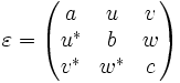
This allows your dielectric to have different dielectric constants for fields polarized in different directions. The epsilon tensor must be positive-definite (have all positive eigenvalues); if it is not, MPB exits with an error. (This does not imply that all of the entries of the epsilon matrix need be positive.) The components of the tensor are specified via three properties:
-
epsilon-diag[vector3] - The diagonal elements (a b c) of the dielectric tensor. No default value.
-
epsilon-offdiag[cvector3] - The off-diagonal elements (u v w) of the dielectric tensor. Defaults to zero. This is a
cvector3, which simply means that the components may be complex numbers (e.g.3+0.1i). If non-zero imaginary parts are specified, then the dielectric tensor is complex-hermitian. This is only supported when MPB is configured with the--with-hermitian-epsflag. This is not dissipative (the eigenvalues of epsilon are real), but rather breaks time-reversal symmetry, corresponding to a gyrotropic (magneto-optic) material. Note that [#inv-symmetry inversion symmetry] may not mean what you expect for complex-hermitian epsilon, so be cautious about usingmpbiin this case. -
epsilon-offdiag-imag[vector3] - Deprecated: The imaginary parts of the off-diagonal elements (u v w) of the dielectric tensor; defaults to zero. Setting the imaginary parts directly by specifying complex numbers in
epsilon-offdiagis preferred.
For example, a material with a dielectric constant of 3.0 for TE fields (polarized in the xy plane) and 5.0 for TM fields (polarized in the z direction) would be specified via (make (dielectric-anisotropic (epsilon-diag 3 3 5))). Please [#tetm-aniso be aware] that not all 2d anisotropic dielectric structures will have TE and TM modes, however.
-
material-function - This material type allows you to specify the material as an arbitrary function of position. (For an example of this, see the
bragg-sine.ctlfile in theexamples/directory.) It has one property:
-
material-func[function] - A function of one argument, the position
vector3(in lattice coordinates), that returns the material at that point.
Note that the function you supply can return any material; wild and crazy users could even return another material-function object (which would then have its function invoked in turn).
Normally, the dielectric constant is required to be positive (or positive-definite, for a tensor). However, MPB does have a somewhat experimental feature allowing negative dielectrics (e.g. in a plasma). To use it, call the function (allow-negative-epsilon) before (run). In this case, it will output the (real) frequency squared in place of the (possibly imaginary) frequencies. (Convergence will be somewhat slower because the eigenoperator is not positive definite.)
geometric-object
This class, and its descendants, are used to specify the solid geometric objects that form the dielectric structure being simulated. The base class is:
-
geometric-object - Properties:
-
material[material-typeclass] - The material that the object is made of (usually some sort of dielectric). No default value (must be specified).
-
center[vector3] - Center point of the object. No default value.
One normally does not create objects of type geometric-object directly, however; instead, you use one of the following subclasses. Recall that subclasses inherit the properties of their superclass, so these subclasses automatically have the material and center properties (which must be specified, since they have no default values).
Recall that all 3-vectors, including the center of an object, its axes, and so on, are specified in the basis of the normalized lattice vectors normalized to basis-size. Note also that 3-vector properties can be specified by either (property (vector3 x y z)) or, equivalently, (property x y z).
In a two-dimensional calculation, only the intersections of the objects with the x-y plane are considered.
-
sphere - A sphere. Properties:
-
radius[number] - Radius of the sphere. No default value.
-
cylinder - A cylinder, with circular cross-section and finite height. Properties:
-
radius[number] - Radius of the cylinder's cross-section. No default value.
-
height[number] - Length of the cylinder along its axis. No default value.
-
axis[vector3] - Direction of the cylinder's axis; the length of this vector is ignored. Defaults to point parallel to the z axis.
-
cone - A cone, or possibly a truncated cone. This is actually a subclass of
cylinder, and inherits all of the same properties, with one additional property. The radius of the base of the cone is given by theradiusproperty inherited fromcylinder, while the radius of the tip is given by the new property:
-
radius2[number] - Radius of the tip of the cone (i.e. the end of the cone pointed to by the
axisvector). Defaults to zero (a "sharp" cone).
-
block - A parallelepiped (i.e., a brick, possibly with non-orthogonal axes). Properties:
-
size[vector3] - The lengths of the block edges along each of its three axes. Not really a 3-vector (at least, not in the lattice basis), but it has three components, each of which should be nonzero. No default value.
-
e1,e2,e3[vector3] - The directions of the axes of the block; the lengths of these vectors are ignored. Must be linearly independent. They default to the three lattice directions.
-
ellipsoid - An ellipsoid. This is actually a subclass of
block, and inherits all the same properties, but defines an ellipsoid inscribed inside the block.
Here are some examples of geometric objects created using the above classes, assuming that the lattice directions (the basis) are just the ordinary unit axes, and m is some material we have defined:
 ; A cylinder of infinite radius and height 0.25 pointing along the x axis,
 ; centered at the origin:
 (make cylinder (center 0 0 0) (material m)
                (radius infinity) (height 0.25) (axis 1 0 0))

 ; An ellipsoid with its long axis pointing along (1,1,1), centered on
 ; the origin (the other two axes are orthogonal and have equal
 ; semi-axis lengths):
 (make ellipsoid (center 0 0 0) (material m)
                 (size 0.8 0.2 0.2)
                (e1 1 1 1)
                (e2 0 1 -1)
                (e3 -2 1 1))

 ; A unit cube of material m with a spherical air hole of radius 0.2 at
 ; its center, the whole thing centered at (1,2,3):
 (set! geometry (list
                (make block (center 1 2 3) (material m) (size 1 1 1))
                (make sphere (center 1 2 3) (material air) (radius 0.2))))
Functions
Here, we describe the functions that are defined by the Photonic-Bands package. There are many types of functions defined, ranging from utility functions for duplicating geometric objects to run functions that start the computation.
See also the reference section of the libctl manual, which describes a number of useful functions defined by libctl.
Geometry utilities
Some utility functions are provided to help you manipulate geometric objects:
-
(shift-geometric-object obj shift-vector) - Translate
objby the 3-vectorshift-vector. -
(geometric-object-duplicates shift-vector min-multiple max-multiple obj) - Return a list of duplicates of
obj, shifted by various multiples ofshift-vector(frommin-multipletomax-multiple, inclusive, in steps of 1). -
(geometric-objects-duplicates shift-vector min-multiple max-multiple obj-list) - Same as
geometric-object-duplicates, except operates on a list of objects,obj-list. If A appears before B in the input list, then all the duplicates of A appear before all the duplicates of B in the output list. -
(geometric-objects-lattice-duplicates obj-list [ ux uy uz ]) - Duplicates the objects in
obj-listby multiples of the lattice basis vectors, making all possible shifts of the "primitive cell" (see below) that fit inside the lattice cell. (This is useful for supercell calculations; see the [user-tutorial.html tutorial].) The primitive cell to duplicate isuxbyuybyuz, in units of the basis vectors. These three parameters are optional; any that you do not specify are assumed to be1. -
(point-in-object? point obj) - Returns whether or not the given 3-vector
pointis inside the geometric objectobj. -
(point-in-periodic-object? point obj) - As
point-in-object?, but also checks translations of the given object by the lattice vectors. -
(display-geometric-object-info indent-by obj) - Outputs some information about the given
obj, indented byindent-byspaces.
Coordinate conversion functions
The following functions allow you to easily convert back and forth between the lattice, cartesian, and reciprocal bases. (See also the [user-tutorial.html#units note on units] in the tutorial.)
-
(lattice->cartesian x),(cartesian->lattice x) - Convert
xbetween the lattice basis (the basis of the lattice vectors normalized tobasis-size) and the ordinary cartesian basis, wherexis either avector3or amatrix3x3, returning the transformed vector/matrix. In the case of a matrix argument, the matrix is treated as an operator on vectors in the given basis, and is transformed into the same operator on vectors in the new basis. -
(reciprocal->cartesian x),(cartesian->reciprocal x) - Like the above, except that they convert to/from reciprocal space (the basis of the reciprocal lattice vectors). Also, the cartesian vectors output/input are in units of 2π.
-
(reciprocal->lattice x),(lattice->reciprocal x) - Convert between the reciprocal and lattice bases, where the conversion again leaves out the factor of 2π (i.e. the lattice-basis vectors are assumed to be in units of 2π).
Also, a couple of rotation functions are defined, for convenience, so that you don't have to explicitly convert to cartesian coordinates in order to use libctl's rotate-vector3 function (see the libctl reference):
-
(rotate-lattice-vector3 axis theta v),(rotate-reciprocal-vector3 axis theta v) - Like
rotate-vector3, except thataxisandvare specified in the lattice/reciprocal bases.
Usually, k-points are specified in the first Brillouin zone, but sometimes it is convenient to specify an arbitrary k-point. However, the accuracy of MPB degrades as you move farther from the first Brillouin zone (due to the choice of a fixed planewave set for a basis). This is easily fixed: simply transform the k-point to a corresponding point in the first Brillouin zone, and a completely equivalent solution (identical frequency, fields, etcetera) is obtained with maximum accuracy. The following function accomplishes this:
-
(first-brillouin-zone k) - Given a k-point
k(in the basis of the reciprocal lattice vectors, as usual), return an equivalent point in the first Brillouin zone of the current lattice (geometry-lattice).
Note that first-brillouin-zone can be applied to the entire k-points list with the Scheme expression: (map first-brillouin-zone k-points).
Run functions
These are functions to help you run and control the simulation. The ones you will most commonly use are the run function and its variants. The syntax of these functions, and one lower-level function, is:
-
(run band-func ...) - This runs the simulation described by the input parameters (see above), with no constraints on the polarization of the solution. That is, it reads the input parameters, initializes the simulation, and solves for the requested eigenstates of each k-point. The dielectric function is outputted to "
epsilon.h5" before any eigenstates are computed.runtakes as arguments zero or more "band functions"band-func. A band function should be a function of one integer argument, the band index, so that(band-func which-band)performs some operation on the bandwhich-band(e.g. outputting fields). After every k-point, each band function is called for the indices of all the bands that were computed. Alternatively, a band function may be a "thunk" (function of zero arguments), in which case(band-func)is called exactly once per k-point. -
(run-zeven band-func ...), (run-zodd band-func ...) - These are the same as the
runfunction except that they constrain their solutions to have even and odd symmetry with respect to the z=0 plane. You should use these functions only for structures that are symmetric through the z=0 mirror plane, where the third basis vector is in the z direction (0,0,1) and is orthogonal to the other two basis vectors, and when the k vectors are in the xy plane. Under these conditions, the eigenmodes always have either even or odd symmetry. In two dimensions, even/odd parities are equivalent to TE/TM polarizations, respectively (and are often strongly analogous even in 3d). Such a symmetry classification is useful for structures such as waveguides and photonic-crystal slabs. (For example, see the paper by S. G. Johnson et al., "Guided modes in photonic crystal slabs," PRB 60, 5751, August 1999.) -
(run-te band-func ...), (run-tm band-func ...) - These are the same as the
runfunction except that they constrain their solutions to be TE- and TM-polarized, respectively, in two dimensions. The TE and TM polarizations are defined has having electric and magnetic fields in the xy plane, respectively. Equivalently, the H/E field of TE/TM light has only a z component (making it easier to visualize).
These functions are actually equivalent to calling run-zeven and run-zodd, respectively.
Note that for the modes to be segregated into TE and TM polarizations, the dielectric function must have mirror symmetry for reflections through the xy plane. If you use [#dielectric-anisotropic anisotropic dielectrics], you should be aware that they break this symmetry if the z direction is not one of the principle axes. If you use run-te or run-tm in such a case of broken symmetry, MPB will exit with an error.
-
(run-yeven band-func ...), (run-yodd band-func ...) - These functions are analogous to
run-zevenandrun-zodd, except that they constrain their solutions to have even and odd symmetry with respect to the y=0 plane. You should use these functions only for structures that are symmetric through the y=0 mirror plane, where the second basis vector is in the y direction (0,1,0) and is orthogonal to the other two basis vectors, and when the k vectors are in the xz plane. -
run-yeven-zeven,run-yeven-zodd,run-yodd-zeven,run-yodd-zodd,run-te-yeven,run-te-yodd,run-tm-yeven,run-tm-yodd - These
run-like functions combine theyeven/yoddconstraints withzeven/zoddorte/tm. See alsorun-parity, below. -
(run-parity p reset-fields band-func ...) - Like the
runfunction, except that it takes two extra parameters, a paritypand a boolean (true/false) valuereset-fields.pspecifies a parity constraint, and should be one of the predefined variables:-
NO-PARITY: equivalent torun -
EVEN-Z(orTE): equivalent torun-zevenorrun-te -
ODD-Z(orTM): equivalent torun-zoddorrun-tm -
EVEN-Y(likeEVEN-Zbut for y=0 plane) -
ODD-Y(likeODD-Zbut for y=0 plane)
-
It is possible to specify more than one symmetry constraint simultaneously by adding them, e.g. (+ EVEN-Z ODD-Y) requires the fields to be even through z=0 and odd through y=0. It is an error to specify incompatible constraints (e.g. (+ EVEN-Z ODD-Z)). Important: if you specify the z/y parity, the dielectric structure (and the k vector) must be symmetric about the z/y=0 plane, respectively.
If reset-fields is false, the fields from any previous calculation will be reused as the starting point from this calculation, if possible; otherwise, the fields are reset to random values. The ordinary run functions use a default reset-fields oftrue. Alternatively, reset-fields may be a string, the name of an HDF5 file to load the initial fields from (as exported by save-eigenvectors, [#eigen-fields below]).
-
(display-eigensolver-stats) - Display some statistics on the eigensolver convergence; this function is useful mainly for MPB developers in tuning the eigensolver.
Several band functions for outputting the eigenfields are defined for your convenience, and are described in the Band output functions section, below. You can also define your own band functions, and for this purpose the functions described in the section Field manipulation functions, below, are useful. A band function takes the form:
(define (my-band-func which-band)
  ...do stuff here with band index which-band...
)
Note that the output variable freqs may be used to retrieve the frequency of the band (see above). Also, a global variable current-k is defined holding the current k-point vector from the k-points list.
There are also some even lower-level functions that you can call, although you should not need to do most of the time:
-
(init-params p reset-fields?) - Read the input variables and initialize the simulation in preparation for computing the eigenvalues. The parameters are the same as the first two parameters of
run-parity. This function must be called before any of the other simulation functions below. (Note, however, that therunfunctions all callinit-params.) -
(set-parity p) - After calling
init-params, you can change the parity constraint without resetting the other parameters by calling this function. Beware that this does not randomize the fields (see below); you don't want to try to solve for, say, the TM eigenstates when the fields are initialized to TE states from a previous calculation. -
(randomize-fields) - Initialize the fields to random values.
-
(solve-kpoint k) - Solve for the requested eigenstates at the Bloch wavevector
k.
The inverse problem: k as a function of frequency
MPB's (run) function(s) and its underlying algorithms compute the frequency w as a function of wavevector k. Sometimes, however, it is desirable to solve the inverse problem, for k at a given frequency w. This is useful, for example, when studying coupling in a waveguide between different bands at the same frequency (frequency is conserved even when wavevector is not). One also uses k(w) to construct wavevector diagrams, which aid in understanding diffraction (e.g. negative-diffraction materials and super-prisms). To solve such problems, therefore, we provide the find-k function described below, which inverts w(k) via a few iterations of Newton's method (using the [#group-vel group velocity] dw/dk). Because it employs a root-finding method, you need to specify bounds on k and a crude initial guess (order of magnitude is usually good enough).
-
(find-k p omega band-min band-max kdir tol kmag-guess kmag-min kmag-max [band-func...]) - Find the wavevectors in the current geometry/structure for the bands from
band-mintoband-maxat the frequencyomegaalong thekdirdirection in k-space. Returns a list of the wavevector magnitudes for each band; the actual wavevectors are(vector3-scale magnitude (unit-vector3 kdir)). The arguments offind-kare:-
p: parity (same as first argument torun-parity, [#run above]). -
omega: the frequency at which to find the bands -
band-min,band-max: the range of bands to solve for the wavevectors of (inclusive). -
kdir: the direction in k-space in which to find the wavevectors. (The magnitude ofkdiris ignored.) -
tol: the fractional tolerance with which to solve for the wavevector;1e-4is usually sufficient. (Like thetoleranceinput variable, this is only the tolerance of the numerical iteration...it does not have anything to do with e.g. the error from finite gridresolution.) -
kmag-guess: an initial guess for the k magnitude (alongkdir) of the wavevector atomega. Can either be a list (one guess for each band fromband-mintoband-max) or a single number (same guess for all bands, which is usually sufficient). -
kmag-min,kmag-max: a range of k magnitudes to search; should be large enough to include the correct k values for all bands. -
band-func: zero or more [#band-funcs band functions], just as in(run), which are evaluated at the computed k points for each band.
-
The find-k routine also prints a line suitable for grepping:
kvals: omega, band-min, band-max, kdir1, kdir2, kdir3, k magnitudes...
Band/output functions
All of these are functions that, given a band index, output the corresponding field or compute some function thereof (in the primitive cell of the lattice). They are designed to be passed as band functions to the run routines, although they can also be called directly. See also the section on [#field-norm field normalizations].
-
(output-hfield which-band) -
(output-hfield-x which-band) -
(output-hfield-y which-band) -
(output-hfield-z which-band) - Output the magnetic (H) field for
which-band; either all or one of the (Cartesian) components, respectively. -
(output-dfield which-band) -
(output-dfield-x which-band) -
(output-dfield-y which-band) -
(output-dfield-z which-band) - Output the electric displacement (D) field for
which-band; either all or one of the (Cartesian) components, respectively. -
(output-efield which-band) -
(output-efield-x which-band) -
(output-efield-y which-band) -
(output-efield-z which-band) - Output the electric (E) field for
which-band; either all or one of the (Cartesian) components, respectively. -
(output-hpwr which-band) - Output the time-averaged magnetic-field energy density (hpwr =
 for
for which-band. -
(output-dpwr which-band) - Output the time-averaged electric-field energy density (dpwr =
 ) for
) for which-band. -
(fix-hfield-phase which-band) -
(fix-dfield-phase which-band) -
(fix-efield-phase which-band) - Fix the phase of the given eigenstate in a canonical way based on the given spatial field (see also
fix-field-phase, below). Otherwise, the phase is random; these functions also maximize the real part of the given field so that one can hopefully just visualize the real part. To fix the phase for output, pass one of these functions torunbefore the corresponding output function, e.g.(run-tm fix-dfield-phase output-dfield-z)
Although we try to maximize the "real-ness" of the field, this has a couple of limitations. First, the phase of the different field components cannot, of course, be chosen independently, so an individual field component may still be imaginary. Second, if you use mpbi to take advantage of [#inv-symmetry inversion symmetry] in your problem, the phase is mostly determined elsewhere in the program; fix-_field-phase in that case only determines the sign.
See also below for the output-poynting and output-tot-pwr functions to output the Poynting vector and the total electromagnetic energy density, respectively.
Sometimes, you only want to output certain bands. For example, here is a function that, given an band/output function like the ones above, returns a new output function that only calls the first function for bands with a large fraction of their energy in an object(s). (This is useful for picking out defect states in supercell calculations.)
-
(output-dpwr-in-objects band-func min-energy objects...) - Given a band function
band-func, returns a new band function that only callsband-funcfor bands having a fraction of their electric-field energy greater thanmin-energyinside the given objects (zero or more geometric objects). Also, for each band, prints the fraction of their energy in the objects in the following form (suitable for grepping):
dpwr:, band-index, frequency, energy-in-objects
output-dpwr-in-objects only takes a single band function as a parameter, but if you want it to call several band functions, you can easily combine them into one with the following routine:
-
(combine-band-functions band-funcs...) - Given zero or more band functions, returns a new band function that calls all of them in sequence. (When passed zero parameters, returns a band function that does nothing.)
It is also often useful to output the fields only at a certain k-point, to let you look at typical field patterns for a given band while avoiding gratuitous numbers of output files. This can be accomplished via:
-
(output-at-kpoint k-point band-funcs...) - Given zero or more band functions, returns a new band function that calls all of them in sequence, but only at the specified
k-point. For other k-points, does nothing.
Miscellaneous functions
-
(retrieve-gap lower-band) - Return the frequency gap from the band #
lower-bandto the band #(lower-band+1), as a percentage of mid-gap frequency. The "gap" may be negative if the maximum of the lower band is higher than the minimum of the upper band. (The gap is computed from theband-range-dataof the previous run.)
Parity
Given a set of eigenstates at a k-point, MPB can compute their parities with respect to the z=0 or y=0 plane. The z/y parity of a state is defined as the expectation value (under the usual inner product) of the mirror-flip operation through z/y=0, respectively. For true even and odd eigenstates (see e.g. run-zeven and run-zodd), this will be +1 and -1, respectively; for other states it will be something in between.
This is useful e.g. when you have a nearly symmetric structure, such as a waveguide with a substrate underneath, and you want to tell which bands are even-like (parity > 0) and odd-like (parity < 0). Indeed, any state can be decomposed into purely even and odd functions, with absolute-value-squared amplitudes of (1+parity)/2 and (1-parity)/2, respectively.
-
display-zparities,display-yparities - These are band functions, designed to be passed to
(run), which output all of the z/y parities, respectively, at each k-point (in comma-delimited format suitable for grepping). -
(compute-zparities) - Returns a list of the parities about the z=0 plane, one number for each band computed at the last k-point.
-
(compute-yparities) - Returns a list of the parities about the y=0 plane, one number for each band computed at the last k-point.
(The reader should recall that the magnetic field is only a pseudo-vector, and is therefore multiplied by -1 under mirror-flip operations. For this reason, the magnetic field appears to have opposite symmetry from the electric field, but is really the same.)
Group velocities
Given a set of eigenstates at a given k-point, MPB can compute their group velocities (the derivative  of frequency with respect to wavevector) using the Hellman-Feynmann theorem. Three functions are provided for this purpose, and we document them here from highest-level to lowest-level.
-
display-group-velocities - This is a band function, designed to be passed to
(run), which outputs all of the group velocity vectors (in the Cartesian basis, in units of c) at each k-point. -
(compute-group-velocities) - Returns a list of group-velocity vectors (in the Cartesian basis, units of c) for the bands at the last-computed k-point.
-
(compute-group-velocity-component direction) - Returns a list of the group-velocity components (units of c) in the given direction, one for each band at the last-computed k-point. direction is a vector in the reciprocal-lattice basis (like the k-points); its length is ignored. (This has the advantage of being three times faster than
compute-group-velocities.)
Field manipulation
The Photonic-Bands package provides a number of ways to take the field of a band and manipulate, process, or output it. These methods usually work in two stages. First, one loads a field into memory (computing it in position space) by calling one of the get functions below. Then, other functions can be called to transform or manipulate the field.
The simplest class of operations involve only the currently-loaded field, which we describe in the [#cur-field second subsection] below. To perform more sophisticated operations, involving more than one field, one must copy or transform the current field into a new field variable, and then call one of the functions that operate on multiple field variables (described in the [#mult-fields third subsection]).
Field normalization
In order to perform useful operations on the fields, it is important to understand how they are normalized. We normalize the fields in the way that is most convenient for perturbation and coupled-mode theory [c.f. SGJ et al., PRE 65, 066611 (2002)], so that their energy densities have unit integral. In particular, we normalize the electric ( ), displacement (
 ) and magnetic (
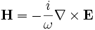 ) fields, so that:
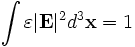
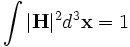
where the integrals are over the computational cell. Note the volume element  (the volume of a grid pixel/voxel). If you simply sum over all the grid points, therefore, you will get (# grid points) / (volume of cell).
Note that we have dropped the pesky factors of 1/2, π, etcetera from the energy densities, since these do not appear in e.g. perturbation theory, and the fields have arbitrary units anyway. The functions to compute/output energy densities below similarly use and without any prefactors.
Loading and manipulating the current field
In order to load a field into memory, call one of the get functions follow. They should only be called after the eigensolver has run (or after init-params, in the case of get-epsilon). One normally calls them after run, or in one of the band functions passed to run.
-
(get-hfield which-band) - Loads the magnetic (H) field for the band
which-band. -
(get-dfield which-band) - Loads the electric displacement (D) field for the band
which-band. -
(get-efield which-band) - Loads the electric (E) field for the band
which-band. (This function actually callsget-dfieldfollowed byget-efield-from-dfield, below.) -
(get-epsilon) - Loads the dielectric function.
Once loaded, the field can be transformed into another field or a scalar field:
-
(get-efield-from-dfield) - Multiplies by the inverse dielectric tensor to compute the electric field from the displacement field. Only works if a D field has been loaded.
-
(fix-field-phase) - Fix the currently-loaded eigenstate's phase (which is normally random) in a canonical way, based on the spatial field (H, D, or E) that has currently been loaded. The phase is fixed to make the real part of the spatial field as big as possible (so that you can hopefully visualize just the real part of the field), and a canonical sign is chosen. See also the
fix-*field-phaseband functions, above, which are convenient wrappers aroundfix-field-phase -
(compute-field-energy) - Given the H or D fields, computes the corresponding energy density function (normalized by the total energy in H or D, respectively). Also prints the fraction of the field in each of its cartesian components in the following form (suitable for grepping):
f-energy-components:, k-index, band-index, x-fraction, y-fraction, z-fraction
where f is either h or d. The return value of compute-field-energy is a list of 7 numbers: (U xr xi yr yi zr zi). U is the total, unnormalized energy, which is in arbitrary units deriving from the normalization of the eigenstate (e.g. the total energy for H is always 1.0). xr is the fraction of the energy in the real part of the field's x component, xi is the fraction in the imaginary part of the x component, etcetera (yr + yi = y-fraction, and so on).
Various integrals and other information about the eigenstate can be accessed by the following functions, useful e.g. for perturbation theory. Functions dealing with the field vectors require a field to be loaded, and functions dealing with the energy density require an energy density to be loaded via compute-field-energy.
-
(compute-energy-in-dielectric min-eps max-eps) - Returns the fraction of the energy that resides in dielectrics with epsilon in the range
min-epstomax-eps. -
(compute-energy-in-objects objects...) - Returns the fraction of the energy inside zero or more geometric objects.
-
(compute-energy-integral f) -
fis a function(f u eps r)that returns a number given three parameters:u, the energy density at a point;eps, the dielectric constant at the same point; andr, the position vector (in lattice coordinates) of the point.compute-energy-integralreturns the integral offover the unit cell. (The integral is computed simply as the sum over the grid points times the volume of a grid pixel/voxel.) This can be useful e.g. for perturbation-theory calculations. -
(compute-field-integral f) - Like
compute-energy-integral, butfis a function(f F eps r)that returns a number (possibly complex) whereFis the complex field vector at the given point. -
(get-epsilon-point r) - Given a position vector
r(in lattice coordinates), return the interpolated dielectric constant at that point. (Since MPB uses a an effective dielectric tensor internally, this actually returns the mean dielectric constant.) -
(get-epsilon-inverse-tensor-point r) - Given a position vector
r(in lattice coordinates), return the interpolated inverse dielectric tensor (a 3x3 matrix) at that point. (Near a dielectric interface, the effective dielectric constant is a tensor even if you input only scalar dielectrics; see the [developer.html#epsilon epsilon overview] for more information.) The returned matrix may be complex-Hermetian if you are employing magnetic materials. -
(get-energy-point r) - Given a position vector
r(in lattice coordinates), return the interpolated energy density at that point. -
(get-field-point r) - Given a position vector
r(in lattice coordinates), return the interpolated (complex) field vector at that point. -
(get-bloch-field-point r) - Given a position vector
r(in lattice coordinates), return the interpolated (complex) Bloch field vector at that point (this is the field without the exp(ikx) envelope).
Finally, we have the following functions to output fields (either the vector fields, the scalar energy density, or epsilon), with the option of outputting several periods of the lattice.
-
(output-field [ nx [ ny [ nz ] ] ]) -
(output-field-x [ nx [ ny [ nz ] ] ]) -
(output-field-y [ nx [ ny [ nz ] ] ]) -
(output-field-z [ nx [ ny [ nz ] ] ]) - Output the currently-loaded field. The optional (as indicated by the brackets) parameters
nx,ny, andnzindicate the number of periods to be outputted along each of the three lattice directions. Omitted parameters are assumed to be 1. For vector fields,output-fieldoutputs all of the (Cartesian) components, while the other variants output only one component. -
(output-epsilon [ nx [ ny [ nz ] ] ]) - A shortcut for calling
get-epsilonfollowed byoutput-field. Note that, because epsilon is a tensor, a number of datasets are outputted in"epsilon.h5":-
"data": 3/trace(1/epsilon) -
"epsilon.{xx,xy,xz,yy,yz,zz}": the (Cartesian) components of the (symmetric) dielectric tensor. -
"epsilon_inverse.{xx,xy,xz,yy,yz,zz}": the (Cartesian) components of the (symmetric) inverse dielectric tensor.
-
Storing and combining multiple fields
In order to perform operations involving multiple fields, e.g. computing the Poynting vector  , they must be stored in field variables. Field variables come in two flavors, real-scalar (rscalar) fields, and complex-vector (cvector) fields. There is a pre-defined field variable
 cur-field representing the currently-loaded field (see above), and you can "clone" it to create more field variables with one of:
-
(field-make f) - Return a new field variable of the same type and size as the field variable
f. Does not copy the field contents (seefield-copyandfield-set!, below). -
(rscalar-field-make f) -
(cvector-field-make f) - Like
field-make, but return a real-scalar or complex-vector field variable, respectively, of the same size asfbut ignoringf's type. -
(field-set! fdest fsrc) - Set
fdestto store the same field values asfsrc, which must be of the same size and type. -
(field-copy f) - Return a new field variable that is exact copy of
f; this is equivalent to callingfield-makefollowed byfield-set!. -
(field-load f) - Loads the field
fas the current field, at which point you can use all of the functions in the [#cur-field previous section] to operate on it or output it.
Once you have stored the fields in variables, you probably want to compute something with them. This can be done in three ways: combining fields into new fields with field-map! (e.g. combine E and H to ), integrating some function of the fields with integrate-fields (e.g. to compute coupling integrals for perturbation theory), and getting the field values at arbitrary points with *-field-get-point (e.g. to do a line or surface integral). These three functions are described below:
-
(field-map! fdest func [f1 f2 ...]) - Compute the new field
fdestto be(func f1-val f2-val ...)at each point in the grid, wheref1-valetcetera is the corresponding value off1etcetera. All the fields must be of the same size, and the argument and return types offuncmust match those of thef1...andfdestfields, respectively.fdestmay be the same field as one of thef1...arguments. Note: all fields are without Bloch phase factors exp(ikx). -
(integrate-fields func [f1 f2 ...]) - Compute the integral of the function
(func r [f1 f2 ...])over the computational cell, whereris the position (in the usual lattice basis) andf1etc. are fields (which must all be of the same size). (The integral is computed simply as the sum over the grid points times the volume of a grid pixel/voxel.) Note: all fields are without Bloch phase factors exp(ikx). See also the note [#mult-fields-bloch below]. -
(cvector-field-get-point f r) -
(cvector-field-get-point-bloch f r) -
(rscalar-field-get-point f r) - Given a position vector
r(in lattice coordinates), return the interpolated field cvector/rscalar fromfat that point.cvector-field-get-point-blochreturns the field without the exp(ikx) Bloch wavevector, in analogue toget-bloch-field-point.
You may be wondering how to get rid of the field variables once you are done with them: you don't, since they are garbage collected automatically.
We also provide functions, in analogue to e.g get-efield and output-efield above, to "get" various useful functions as the [#cur-field current field] and to output them to a file:
-
(get-poynting which-band) - Loads the Poynting vector E*xH for the band
which-band, the flux density of electromagnetic energy flow, as the current field. 1/2 of the real part of this vector is the time-average flux density (which can be combined with the imaginary part to determine the amplitude and phase of the time-dependent flux). -
(output-poynting which-band) -
(output-poynting-x which-band) -
(output-poynting-y which-band) -
(output-poynting-z which-band) - Output the Poynting vector field for
which-band; either all or one of the (Cartesian) components, respectively. -
(get-tot-pwr which-band) - Load the time-averaged electromgnetic-field energy density (|H|2 + epsilon*|E|2) for
which-band. (If you multiply the real part of the Poynting vector by a factor of 1/2, above, you should multiply by a factor of 1/4 here for consistency.) -
(output-tot-pwr which-band) - Output the time-averaged electromgnetic-field energy density (above) for
which-band.
As an example, below is the Scheme source code for the get-poynting function, illustrating the use of the various field functions:
(define (get-poynting which-band)
  (get-efield which-band)                      ; put E in cur-field
  (let ((e (field-copy cur-field)))            ; ... and copy to local var.
    (get-hfield which-band)                    ; put H in cur-field
    (field-map! cur-field                      ; write ExH to cur-field
                (lambda (e h) (vector3-cross (vector3-conj e) h))
                e cur-field)
    (cvector-field-nonbloch! cur-field)))      ; see below
Stored fields and Bloch phases
Complex vector fields like E and H as computed by MPB are physically of the Bloch form: exp(ikx) times a periodic function. What MPB actually stores, however, is just the periodic function, the Bloch envelope, and only multiplies by exp(ikx) for when the fields are output or passed to the user (e.g. in integration functions). This is mostly transparent, with a few exceptions noted above for functions that do not include the exp(ikx) Bloch phase (it is somewhat faster to operate without including the phase).
On some occasions, however, when you create a field with field-map!, the resulting field should not have any Bloch phase. For example, for the Poynting vector E*xH, the exp(ikx) cancels because of the complex conjugation. After creating this sort of field, we must use the special function cvector-field-nonbloch! to tell MPB that the field is purely periodic:
-
(cvector-field-nonbloch! f) - Specify that the field
fis not of the Bloch form, but rather that it is purely periodic.
Currently, all fields must be either Bloch or non-Bloch (i.e. periodic), which covers most physically meaningful possibilities.
There is another wrinkle: even for fields in Bloch form, the exp(ikx) phase currently always uses the current k-point, even if the field was computed from another k-point. So, if you are performing computations combining fields from different k-points, you should take care to always use the periodic envelope of the field, putting the Bloch phase in manually if necessary.
Manipulating the raw eigenvectors
MPB also includes a few low-level routines to manipulate the raw eigenvectors that it computes in a transverse planewave basis.
The most basic operations involve copying, saving, and restoring the current set of eigenvectors or some subset thereof:
-
(get-eigenvectors first-band num-bands) - Return an eigenvector object that is a copy of
num-bandscurrent eigenvectors starting atfirst-band. e.g. to get a copy of all of the eigenvectors, use(get-eigenvectors 1 num-bands). -
(set-eigenvectors ev first-band) - Set the current eigenvectors, starting at
first-band, to those in theeveigenvector object (as returned byget-eigenvectors). (Does not work if the grid sizes don't match) -
(load-eigenvectors filename) -
(save-eigenvectors filename) - Read/write the current eigenvectors (raw planewave amplitudes) to/from an HDF5 file named
filename. Instead of usingload-eigenvectorsdirectly, you can pass thefilenameas thereset-fieldsparameter ofrun-parity, [#run above]. (Loaded eigenvectors must be of the same size (same grid size and #bands) as the current settings.)
Currently, there's only one other interesting thing you can do with the raw eigenvectors, and that is to compute the dot-product matrix between a set of saved eigenvectors and the current eigenvectors. This can be used, e.g., to detect band crossings or to set phases consistently at different k points. The dot product is returned as a "sqmatrix" object, whose elements can be read with the sqmatrix-size and sqmatrix-ref routines.
-
(dot-eigenvectors ev first-band) - Returns a sqmatrix object containing the dot product of the saved eigenvectors
evwith the current eigenvectors, starting atfirst-band. That is, the (i,j)th output matrix element contains the dot product of the (i+1)th vector ofev(conjugated) with the (first-band+j)th eigenvector. Note that the eigenvectors, when computed, are orthonormal, so the dot product of the eigenvectors with themselves is the identity matrix. -
(sqmatrix-size sm) - Return the size n of an nxn sqmatrix
sm. -
(sqmatrix-ref sm i j) - Return the (
i,j)th element of the nxn sqmatrixsm, where {i,j} range from 0..n-1.
Inversion Symmetry
If you configure MPB with the --with-inv-symmetry flag, then the program is configured to assume inversion symmetry in the dielectric function. This allows it to run at least twice as fast and use half as much memory as the more general case. This version of MPB is by default installed as mpbi, so that it can coexist with the usual mpb program.
Inversion symmetry means that if you transform (x,y,z) to (-x,-y,-z) in the coordinate system, the dielectric structure is not affected. Or, more technically, that:
where the conjugation is significant for [#dielectric-anisotropic complex-hermitian dielectric tensors]. This symmetry is very common; all of the examples in this manual have inversion symmetry, for example.
Note that inversion symmetry is defined with respect to a specific origin, so that you may "break" the symmetry if you define a given structure in the wrong way--this will prevent mpbi from working properly. For example, the [analysis-tutorial.html#diamond diamond structure] that we considered earlier would not have possessed inversion symmetry had we positioned one of the "atoms" to lie at the origin.
You might wonder what happens if you pass a structure lacking inversion symmetry to mpbi. As it turns out, mpbi only looks at half of the structure, and infers the other half by the inversion symmetry, so the resulting structure always has inversion symmetry, even if its original description did not. So, you should be careful, and look at the epsilon.h5 output to make sure it is what you expected.
Parallel MPB
We provide two methods by which you can parallelize MPB. The first, using MPI, is the most sophisticated and potentially provides the greatest and most general benefits. The second, which involves a simple script to split e.g. the k-points list among several processes, is less general but may be useful in many cases.
MPB with MPI parallelization
If you configure MPB with the --with-mpi flag, then the program is compiled to take advantage of distributed-memory parallel machines with MPI, and is installed as mpb-mpi. (See also the [installation.html#mpi installation section].) This means that computations will (potentially) run more quickly and take up less memory per processor than for the serial code.
Using the parallel MPB is almost identical to using the serial version(s), with a couple of minor exceptions. The same ctl files should work for both. Running a program that uses MPI requires slightly different invocations on different systems, but will typically be something like:
unix% mpirun -np 4 mpb-mpi foo.ctl
to run on e.g. 4 processors. A second difference is that 1D systems are currently not supported in the MPI code, but the serial code should be fast enough for those anyway. A third difference is that the output HDF5 files (epsilon, fields, etcetera) from mpb-mpi have their first two dimensions (x and y) transposed; i.e. they are output as YxXxZ arrays. This doesn't prevent you from visualizing them, but the coordinate system is left-handed; to un-transpose the data, you can process it with mpb-data and the -T option (in addition to any other options).
In order to get optimal benefit (time and memory savings) from mpb-mpi, the first two dimensions (nx and ny) of your grid should both be divisible by the number of processes. If you violate this constraint, MPB will still work, but the load balance between processors will be uneven. At worst, e.g. if either nx or ny is smaller than the number of processes, then some of the processors will be idle for part (or all) of the computation. When using [#inv-symmetry inversion symmetry] (mpbi-mpi) for 2D grids only, the optimal case is somewhat more complicated: nx and (ny/2 + 1), not ny, should both be divisible by the number of processes.
mpb-mpi divides each band at each k-point between the available processors. This means that, even if you have only a single k-point (e.g. in a defect calculation) and/or a single band, it can benefit from parallelization. Moreover, memory usage per processor is inversely proportional to the number of processors used. For sufficiently large problems, the speedup is also nearly linear.
MPI support in MPB is thanks to generous support from Clarendon Photonics.
Alternative parallelization: mpb-split
There is an alternative method of parallelization when you have multiple k points: do each k-point on a different processor. This does not provide any memory benefits, and does not allow one k-point to benefit by starting with the fields of the previous k-point, but is easy and may be the only effective way to parallelize calculations for small problems. This method also does not require MPI: it can utilize the unmodified serial mpb program. To make it even easier, we supply a simple script called mpb-split (or mpbi-split) to break the k-points list into chunks for you. Running:
unix% mpb-split num-split foo.ctl
will break the k-points list in foo.ctl into num-split more-or-less equal chunks, launch num-split processes of mpb in parallel to process each chunk, and output the results of each in order. (Each process is an ordinary mpb execution, except that it numbers its k-points depending upon which chunk it is in, so that output files will not overwrite one another and you can still grep for frequencies as usual.)
Of course, this will only benefit you on a system where different processes will run on different processors, such as an SMP or a cluster with automatic process migration (e.g. MOSIX). mpb-split is actually a trivial shell script, though, so you can easily modify it if you need to use a special command to launch processes on other processors/machines (e.g. via GNU Queue).
The general syntax for mpb-split is:
unix% mpb-split num-split mpb-arguments...
where all of the arguments following num-split are passed along to mpb. What mpb-split technically does is to set the MPB variable k-split-num to num-split and k-split-index to the index (starting with 0) of the chunk for each process. If you want, you can use these variables to divide the problem in some other way and then reset them to 1 and , respectively.
