The MPB Manual
From AbInitio
Contents
|
Introduction
| |
| MIT Photonic Bands |
| Download |
| Release notes |
| MPB manual |
| Introduction |
| Installation |
| User Tutorial |
| Data Analysis Tutorial |
| User Reference |
| Developer Information |
| Acknowledgements |
| License and Copyright |
MIT Photonic Bands is a software package to compute definite-frequency eigenstates of Maxwell's equations in periodic dielectric structures. Its primary intended application is the study of photonic crystals: periodic dielectric structures exhibiting a band gap in their optical modes, prohibiting propagation of light in that frequency range. However, it could also be easily applied to compute other optical dispersion relations and eigenstates (e.g. for conventional waveguides such as fiber-optic cables).
This manual assumes that the reader is familiar with concepts from solid-state physics such as eigenstates, band structures, and Bloch's theorem. We also do not attempt (much) to instruct the reader on photonic crystals or other optical applications for which this code might be useful. For an excellent introduction to all of these topics in the context of photonic crystals, see the book Photonic Crystals: Molding the Flow of Light, by J. D. Joannopoulos, R. D. Meade, and J. N. Winn (Princeton, 1995).
Some of the main design goals we were thinking about when we developed this package were the following (see also the feature list at the MPB home page):
- Fully vectorial, three-dimensional calculations for arbitrary Bloch wavevectors. (The only approximation is the spatial discretization, or equivalently the planewave cutoff.)
- Flexible interface. Readable, extensible, scriptable...see also the libctl design goals.
- Parallel. (Can run on a single-processor machine, but is also supports parallel machines with MPI.)
- "Targeted" eigensolver: find modes nearest to a specified frequency, not just the lowest-frequency bands. (For defect calculations.)
- Leverage existing software (LAPACK, BLAS, FFTW, HDF, MPI, GUILE...).
- Modularity. The eigensolver, Maxwell's equations, user interface, and so on, should be oblivious to each other as much as possible. This way, they can be debugged separately, combined in various ways, replaced, used in other programs...all the usual benefits of modular design.
- Take advantage of inversion symmetry in the dielectric function, but don't require it. (This means that we have to handle both real and complex fields.)
Frequency-Domain vs. Time-Domain
There are two common computational approaches to studying dielectric structures such as photonic crystals: frequency-domain and time-domain. We feel that each has its own place in a researcher's toolbox, and each has unique advantages and disadvantages (for a more detailed discussion, see our online textbook, appendix D). MPB is frequency-domain; that is, it does a direct computation of the eigenstates and eigenvalues of Maxwell's equations (using a planewave basis). Each field computed has a definite frequency. In contrast, time-domain techniques (as in our Meep software) iterate Maxwell's equations in time; the computed fields have a definite time (at each time step) but not a definite frequency per se. It seems worthwhile to say a few words about each method, and to explain why we want a frequency-domain code. (Our group has both time-domain and frequency-domain software, and we use both techniques extensively.)
Time-domain methods are well-suited to computing things that involve evolution of the fields, such as transmission and resonance decay-time calculations. They can also be used to calculate band structures and for finding resonant modes, by looking for peaks in the Fourier transform of the system response to some input. The main advantage of this is that you get all the frequencies (peaks) at once from a calculation involving propagation of a single field. There are several disadvantages to this technique, however. First, it is hard to be confident that you have found all of the states—you may have coupled weakly to some state by accident, or two states may be close in frequency and appear as a single peak; this is especially problematic in higher-order resonant-cavity and waveguide calculations. Second, in the Fourier transform, the frequency resolution is inversely related to the simulation time; to get 10 times the resolution you must run your simulation 10 times as long (although matters are improved by using more sophisticated signal-processing methods such as Harminv's). Third, the time-step size must be proportional to the spatial-grid size for numerical stability; thus, if you double the spatial resolution, you must double the number of time steps (the length of your simulation), even if you are looking at states with the same frequency as before. Fourth, you only get the frequencies of the states; to get the eigenstates themselves (so that you can see what the modes look like and do calculations with them), you must run the simulation again, once for each state that you want, and for a time inversely proportional to the frequency-spacing between adjacent states (i.e. a long time for closely-spaced states).
In contrast, frequency-domain methods like those in MPB are in many ways better-suited to calculating band structures and eigenstates. (Here, we consider the case of an iterative eigensolver like the one in MPB, which iteratively improves approximate eigenstates. Dense solvers, which factorize the matrix directly, are impractical for large problems because of the huge size of the matrix, and because they compute many more eigenvectors than are desired. In iterative methods, the operator is only applied to individual vectors and is never itself computed explicitly.) First, you don't have to worry about missing states—even closely-spaced modes will appear as two eigenvalues in the result. Second, the error in the frequency in an iterative eigensolver typically decays exponentially with the number of iterations, so the number of iterations is logarithmic in the desired tolerance. Third, the number of iterations typically remains almost constant even as you increase the resolution (the work for each iteration increases, of course, but that happens in time-domain too). Fourth, you get both the frequencies and the eigenstates at the same time, so you can look at the modes immediately (even closely-spaced ones).
A traditional disadvantage of frequency-domain methods was that you had to compute all of the lowest eigenstates, up to the desired one, even if you didn't care about the lower ones. This was especially problematic in defect calculations, in which a large supercell is used, because in that case the lower bands are "folded" many times in the Brillouin zone. Thus, you often had to compute a large number of bands in order to get to the one you wanted (incurring large costs both in time and in storage). These disadvantages disappear to some degree in MPB, however, with the advent of its "targeted" eigensolver—with it, you can solve directly for the localized defect states (i.e the states in the band gap) without computing the lower bands. However, the targeted eigensolver method used in MPB still has poor convergence, so time-domain methods such as Meep still have an advantage here.
History
In order to shed some light on the past development and design decisions of the Photonic-Bands package, I thought I'd write a few paragraphs about its history. Read on to enjoy my narcissistic ramblings.
Many different people have written codes to compute the modes of periodic dielectric materials (although we don't know of any others that have been freely released). I have had experience with several programs written within our group, and this experience has guided the design of MIT Photonic-Bands.
The first program of this sort that I came in contact with, and the code that was used in our group until the development of this package, was initially written around 1990 (in Fortran 77) by R. D. Meade. As this software grew organically over time, several problems became apparent. First, the input format was inflexible (difficult to add new features without breaking old simulations), sensitive to whitespace and other formatting, and required repeated entry of information that was often the same from file to file. Often, pre- and post-processing steps were required using additional scripts and tools. Second, the many parts of the program had become intertwined, lacking modularity or a clear flow of control; this made it difficult to follow or modify substantially. Parallelizing it, or removing constraints that it imposed like inversion symmetry, or even replacing the input format seemed impractical. Besides, even reading code with variables named gxgzco (in common block cabgv) (honest!) is a mind-altering experience.
After an initial experience in the Spring of 1996 at writing a code based on a wavelet, rather than a planewave, basis (which turned out not to be practical), I set out to write a replacement for our Fortran eigensolver. My main aims at this time (Fall 1996) were a more flexible and powerful input format and a code that would be amenable to parallelization. I succeeded in achieving a working code with similar convergence to the old code (after some pain), but I discovered several things. I had lots of fun learning to use lex and yacc (Yet Another Compiler-Compiler) to make a flexible, C-like input format with variables and other advanced features. Having input files that were almost, but not quite, like a programming language made me realize, however, that what I really wanted was a programming language--no matter how many features I added, I always wanted one more "simple" thing. As far as parallelization, I quickly realized that I had a problem: I needed a parallel FFT, and the only ones that were available were proprietary (non-portable), used incompatible data distribution formats, and were often designed to be called only from special languages like HPF. That, plus my dissatisfaction with the available free FFTs, led me to embark on a side project (with my friend Matteo Frigo of MIT's Laboratory for Computer Science) to develop a new, free FFT library, FFTW, that included portable parallel routines. Also, I decided that attempting to support too many models of parallel programming (threads, MPI, Cray shmem) in one program resulted in a mess; it was better to stick with MPI (supporting running only a single process too, of course). Another mistake I discovered was that I allowed the eigensolver to get too intertwined with the specific problem of Maxwell's equations--the eigensolver knew about the data structures for the fields, etcetera, making it difficult to plug in replacement eigensolvers, test things in isolation, or to implement features like the "targeted" eigensolver of Photonic-Bands (which diagonalizes a different operator). The whole program was too mired in complexity. Finally, in the interim I had learned about block eigensolver algorithms. Not only can such algorithms leverage prepackaged, highly-optimized routines like BLAS and LAPACK, but they also promised to be inherently more suited for parallelization (since they remove the serial process of solving for the bands one by one). All of these things convinced me that I needed to rewrite the code again from scratch.
So, I started work on the new package (in Spring 1998), this time determined to develop and debug each component (matrix operations, eigensolver, maxwell operator, user input) in isolation. At the same time, I was thinking about how I would implement the user control language, wanting to develop a general tool that could be applied to other problems and software in our research. It seemed clear that, in order to get other people to use it in their programs, as well as to avoid a lot of the manual labor that went into my previous effort, I wanted to automatically generate the user/program interface from an abstract specification. As for the control language, I briefly considered implementing my own, but was happily led to GNU Guile instead, which gave me a powerful language with little effort. So armed, I set out to write libctl (which generates the Guile interface from an abstract Scheme specification), partially as an experiment to see how hard it would be and what the result would look like. After a weekend of work, it was obvious that I had a powerful tool; I spent couple of weeks adding some finishing touches, writing documentation, and so on, and proudly showed it off to my groupmates in the hope that they could use it for their programs. Without a real example of a program using libctl, however, it was hard to convince them to plug a scripting language into their existing, working codes. So, I went back to puttering at my eigensolvers.
Of course, all this time I was allegedly doing real research, and long periods would go by with little progress on the Photonic-Bands package. The original, Fortran code was still working, and in time one learned to bear its quirks and limitations with stoicism, although we cringed every time we had to show it to anyone else. By the summer of 1999, I had a working block eigensolver (supporting several iteration-scheme variants), a Maxwell operator to plug into the eigensolver (including a "targeted" operator, whose convergence I was unhappy with), and a test program to do convergence experiments on bands of a Bragg mirror. I hadn't attached any general user interface, field output, or other necessary components. At this point, Dr. Doug Allan of Corning (a former student of Prof. Joannopoulos), heard about the new code--in particular, the targeted eigensolver--and began clamoring to try it out. Not put off by my excuses, he asked for a copy of my current code, regardless of its status, to play with. Not wanting to refuse, but aghast at the prospect of someone seeing my masterpiece only half-painted, I told him to give me a week...in which time I added the interface and discovered that I had a useful tool. Over the next week, I added many features, fixed bugs, and wrote documentation, drawing near to a release at last...
Installation
| |
| MIT Photonic Bands |
| Download |
| Release notes |
| MPB manual |
| Introduction |
| Installation |
| User Tutorial |
| Data Analysis Tutorial |
| User Reference |
| Developer Information |
| Acknowledgements |
| License and Copyright |
In this section, we outline the procedure for installing the MIT Photonic-Bands package. Mainly, this consists of downloading and installing various prerequisites. As much as possible, we have attempted to take advantage of existing packages such as BLAS, LAPACK, FFTW, and GNU Guile, in order to make our code smaller, more robust, faster, and more flexible. Unfortunately, this may make the installation of MPB more complicated if you do not already have these packages.
You will also need an ANSI C compiler, of course (gcc is fine), and installation will be easiest on a UNIX-like system (Linux is fine). In the following list, some of the packages are dependent upon packages listed earlier, so you should install them in more-or-less the order given.
Note: Many of these libraries may be available in precompiled binary form, especially for GNU/Linux systems. Be aware, however, that library binary packages often come in two parts, library and library-dev, and both are required to compile programs using it.
Note: It is important that you use the same Fortran compiler to compile Fortran libraries (like LAPACK) and for configuring MPB. Different Fortran compilers often have incompatible linking schemes. (The Fortran compiler for MPB can be set via the F77 environment variable.)
Note: The latest, pre-installed versions of MPB and Meep running on Ubuntu can also be accessed on Amazon Web Services (AWS) Elastic Compute Cloud (EC2) as a free Amazon Machine Image (AMI). To access this AMI, follow these instructions.
Installation on MacOS X
See Meep installation on OS X for the easiest way to do this.
Unix Installation Basics
Installation Paths
First, let's review some important information about installing software on Unix systems, especially in regards to installing software in non-standard locations. (None of these issues are specific to this software, but they've caused a lot of confusion among our beloved users.)
Most of the software below, including this software, installs under /usr/local by default; that is, libraries go in /usr/local/lib, programs in /usr/local/bin, etc. If you don't have root privileges on your machine, you may need to install somewhere else, e.g. under $HOME/install (the install/ subdirectory of your home directory). Most of the programs below use a GNU-style configure script, which means that all you would do to install there would be:
./configure --prefix=$HOME/install
when configuring the program; the directories $HOME/install/lib etc. are created automatically as needed.
Paths for Configuring
There are two further complications. First, if you install in a non-standard location (and /usr/local is considered non-standard by some proprietary compilers), you will need to tell the compilers where to find the libraries and header files that you dutifully installed. You do this by setting two environment variables:
setenv LDFLAGS "-L/usr/local/lib"
setenv CPPFLAGS "-I/usr/local/include"
Of course, substitute whatever installation directory you used. Do this before you run the configure scripts, etcetera. You may need to include multiple -L and -I flags (separated by spaces) if your machine has stuff installed in several non-standard locations. Bourne shell users (e.g. bash or ksh) should use the "export FOO=bar" syntax instead of csh's "setenv FOO bar", of course.
You might also need to update your PATH so that you can run the executables you installed (although /usr/local/bin is in the default PATH on many systems). e.g. if we installed in our home directory as described above, we would do:
setenv PATH "$HOME/install/bin:$PATH"
Paths for Running (Shared Libraries)
Second, many of the packages installed below (e.g. Guile) are installed as shared libraries. You need to make sure that your runtime linker knows where to find these shared libraries. The bad news is that every operating system does this in a slightly different way. The good news is that, when you run make install for the packages involving shared libraries, the output includes the necessary instructions specific to your system, so pay close attention! It will say something like "add LIBDIR to the foobar environment variable," where LIBDIR will be your library installation directory (e.g. /usr/local/lib) and foobar is some environment variable specific to your system (e.g. LD_LIBRARY_PATH on some systems, including Linux). For example, you might do:
setenv LD_LIBRARY_PATH "/usr/local/lib:$LD_LIBRARY_PATH"
Note that we just add to the library path variable, and don't replace it in case it contains stuff already. If you use Linux and have root privileges, you can instead simply run /sbin/ldconfig, first making sure that a line "/usr/local/lib" (or whatever) is in /etc/ld.so.conf.
If you don't want to type these commands every time you log in, you can put them in your ~/.cshrc file (or ~/.profile, or ~/.bash_profile, depending on your shell).
Fun with Fortran
Our software, along with many of the libraries it calls, is written in C or C++, but it also calls libraries such as BLAS and LAPACK (see below) that are usually compiled from Fortran. This can cause some added difficulty because of the various linking schemes used by Fortran compilers. Our configure script attempts to detect the Fortran linking scheme automatically, but in order for this to work you must use the same Fortran compiler and options with our software as were used to compile BLAS/LAPACK.
By default, our software looks for a vendor Fortran compiler first (f77, xlf, etcetera) and then looks for GNU g77. In order to manually specify a Fortran compiler foobar you would configure it with './configure F77=foobar ...'.
If, when you compiled BLAS/LAPACK, you used compiler options that alter the linking scheme (e.g. g77's -fcase-upper or -fno-underscoring), you will need to pass the same flags to our software via './configure FFLAGS="...flags..." ...'.
Picking a compiler
It is often important to be consistent about which compiler you employ. This is especially true for C++ software. To specify a particular C compiler foo, configure with ./configure CC=foo; to specify a particular C++ compiler foo++, configure with ./configure CXX=foo++; to specify a particular Fortran compiler foo90, configure with ./configure F77=foo90.
GNU/Linux and BSD binary packages
If you are installing on your personal GNU/Linux or BSD machine, then precompiled binary packages are likely to be available for many of these packages, and may even have been included with your system. On Debian systems, the packages are in .deb format and the built-in apt-get program can fetch them from a central repository. On Red Hat, SuSE, and most other Linux-based systems, binary packages are in RPM format and can be fetched (if they did not come with your system) from places like rpmfind.net. OpenBSD has its "ports" system, and so on.
Do not compile something from source if an official binary package is available. For one thing, you're just creating pain for yourself. Worse, the binary package may already be installed, in which case installing a different version from source will just cause trouble.
One thing to watch out for is that libraries like LAPACK, Guile, HDF5, etcetera, will often come split up into two (or more) packages: e.g. a guile package and a guile-devel package. You need to install both of these to compile software using the library.
BLAS and LAPACK
MPB requires the BLAS and LAPACK libraries for matrix computations.
BLAS
The first thing you must have on your system is a BLAS implementation. "BLAS" stands for "Basic Linear Algebra Subroutines," and is a standard interface for operations like matrix multiplication. It is designed as a building-block for other linear-algebra applications, and is used both directly by our code and in LAPACK (see below). By using it, we can take advantage of many highly-optimized implementations of these operations that have been written to the BLAS interface. (Note that you will need implementations of BLAS levels 1-3.)
You can find more BLAS information, as well as a basic implementation, on the BLAS Homepage. Once you get things working with the basic BLAS implementation, it might be a good idea to try and find a more optimized BLAS code for your hardware. Vendor-optimized BLAS implementations are available as part of the Intel MKL, HP CXML, IBM ESSL, SGI sgimath, and other libraries. An excellent, high-performance, free-software BLAS implementation is OpenBLAS; another is ATLAS.
Note that the generic BLAS does not come with a Makefile; compile it with something like:
get http://www.netlib.org/blas/blas.tgz
gunzip blas.tgz
tar xf blas.tar
cd BLAS
f77 -c -O3 *.f   # compile all of the .f files to produce .o files
ar rv libblas.a *.o    #  combine the .o files into a library
su -c "cp libblas.a /usr/local/lib"   # switch to root and install
(Replace -O3 with your favorite optimization options. On Linux, I use g77 -O3 -fomit-frame-pointer -funroll-loops, with -malign-double -mcpu=i686 on a Pentium II.) Note that MPB looks for the standard BLAS library with -lblas, so the library file should be called libblas.a and reside in a standard directory like /usr/local/lib. (See also below for the --with-blas=lib option to MPB's configure script, to manually specify a library location.)
LAPACK
LAPACK, the Linear Algebra PACKage, is a standard collection of routines, built on BLAS, for more-complicated (dense) linear algebra operations like matrix inversion and diagonalization. You can download LAPACK from the LAPACK Home Page.
Note that our software looks for LAPACK by linking with -llapack. This means that the library must be called liblapack.a and be installed in a standard directory like /usr/local/lib (alternatively, you can specify another directory via the LDFLAGS environment variable as described earlier). (See also below for the --with-lapack=lib option to our configure script, to manually specify a library location.)
I currently recommend installing OpenBLAS, which includes LAPACK so you do not need to install it separately.
MPI (for parallel MPB)
Optionally, MPB is able to run on a distributed-memory parallel machine, and to do this we use the standard MPI message-passing interface. You can learn about MPI from the MPI Home Page. Most commercial supercomputers already have an MPI implementation installed; two free MPI implementations that you can install yourself are MPICH and LAM; a promising new implementation is Open MPI. MPI is not required to compile the ordinary, uniprocessor version of our software.
In order for the MPI version of our software to run successfully, we have a slightly nonstandard requirement: each process must be able to read from the disk. (This way, Guile can boot for each process and they can all read your control file in parallel.) Many (most?) commercial supercomputers, Linux Beowulf clusters, etcetera, satisfy this requirement.
Also, in order to get good performance, you'll need fast interconnect hardware such as Myrinet; 100Mbps Ethernet probably won't cut it. The speed bottleneck comes from the FFT, which requires most of the communications in MPB. FFTW's MPI transforms (see below) come with benchmark programs that will give you a good idea of whether you can get speedups on your system. Of course, even with slow communications, you can still benefit from the memory savings per CPU for large problems.
As described below, when you configure MPB with MPI support (--with-mpi), it installs itself as mpb-mpi. See also the [user-ref.html#mpb-mpi user reference] section for information on using MPB on parallel machines. Normally, you should also install the serial version of MPB, if only to get the mpb-data utility, which is not installed with the MPI version.
MPI support in MPB is thanks to generous support from Clarendon Photonics.
HDF5 (optional, strongly advised)
We require a portable, standard binary format for outputting the electromagnetic fields and similar volumetric data, and for this we use HDF. (If you don't have HDF5, you can still compile MPB, but you won't be able to output the fields or the dielectric function.)
HDF is a widely-used, free, portable library and file format for multi-dimensional scientific data, developed in the National Center for Supercomputing Applications (NCSA) at the University of Illinois (UIUC, home of the Fighting Illini and alma mater to many of this author's fine relatives). You can get HDF and learn about it on the HDF Home Page.
There are two incompatible versions of HDF, HDF4 and HDF5 (no, not HDF1 and HDF2). We require the newer version, HDF5, which is supported by a number scientific of visualization tools, including our own h5utils utilities.
HDF5 includes parallel I/O support under MPI, which can be enabled by configuring it with --enable-parallel. (You may also have to set the CC environment variable to mpicc.) Unfortunately, the parallel HDF5 library then does not work with serial code, so you have may have to choose one or the other.
We have some hacks in our MPB and Meep software so that they can do parallel I/O even with the serial HDF5 library; these hacks work okay when you are using a small number of processors, but on large supercomputers we strongly recommend using the parallel HDF5.
Note: If you have a version of HDF5 compiled with MPI parallel I/O support, then you need to use the MPI compilers to link to it, even when you are compiling the serial versions of Meep or MPB. Just use ./configure CC=mpicc CXX=mpic++ (or whatever your MPI compilers are) when configuring.
Note: version 1.8 of HDF5 changed the programming interface, breaking older programs like MPB (versions 1.4.x and earlier) and Meep (versions 0.11.x and earlier). As a workaround, if you have HDF5 1.8 or later and would like to compile these versions of MPB and/or Meep, include -DH5_USE_16_API=1 in the CPPFLAGS (see below).
FFTW
FFTW is a self-optimizing, portable, high-performance FFT implementation, including both serial and parallel FFTs. You can download FFTW and find out more about it from the FFTW Home Page.
If you want to use MPB on a parallel machine with MPI, you will also need to install the MPI FFTW libraries (this just means including --enable-mpi in the FFTW configure flags).
GNU Readline (optional)
GNU Readline is a library to provide command-line history, tab-completion, emacs keybindings, and other shell-like niceties to command-line programs. This is an optional package, but one that can be used by Guile (see below) if it is installed; we recommend getting it. You can download Readline from the GNU ftp site. (Readline is typically preinstalled on GNU/Linux systems).
GNU Guile
GNU Guile is an extension/scripting language implementation based on Scheme, and we use it to provide a rich, fully-programmable user interface with minimal effort. It's free, of course, and you can download it from the Guile Home Page. (Guile is typically included with GNU/Linux systems.)
- Important: Most Linux distributions come with Guile already installed (check by seeing whether you can run
guile --versionfrom the command line). In that case, do not install your own version of Guile from source — having two versions of Guile on the same system will cause problems. However, by default most distributions install only the Guile libraries and not the programming headers — to compile libctl and MPB, you should install the "guile-devel" or "guile-dev" package (e.g. with RPM) that came with your system.
GNU Autoconf (optional)
If you want to be a developer of the MPB package (as opposed to merely a user), you will also need the GNU Autoconf program. Autoconf is a portability tool that generates configure scripts to automatically detect the capabilities of a system and configure a package accordingly. You can find out more at the Autoconf Home Page (autoconf is typically installed by default on Linux systems). In order to install Autoconf, you will also need the GNU m4 program if you do not already have it (see the GNU m4 Home Page).
libctl
Instead of using Guile directly, we separated much of the user interface code into a package called libctl, in the hope that this might be more generally useful. libctl automatically handles the communication between the program and Guile, converting complicated data structures and so on, to make it even easier to use Guile to control scientific applications. Download libctl from the libctl page, unpack it, and run the usual configure, make, make install sequence. You'll also want to browse the libctl manual, as this will give you a general overview of what the user interface will be like.
If you are not the system administrator of your machine, and/or want to install libctl somewhere else (like your home directory), you can do so with the standard --prefix=dir option to configure (the default prefix is /usr/local). In this case, however, you'll need to specify the location of the libctl shared files for the MPB or Meep package, using the --with-libctl=dir/share/libctl option to our configure script.
MIT Photonic Bands
Okay, if you've made it all the way here, you're ready to install the MPB package and start cranking out eigenmodes. (You can download the latest version and read this manual at the MIT Photonic-Bands Homepage.) Once you've unpacked it, just run:
./configure
make
to configure and compile the package (see below to install). Hopefully, the configure script will correctly detect the BLAS, FFTW, etcetera libraries that you've dutifully installed, as well as the C compiler and so on, and the make compilation will proceed without a hitch. If not, it's a Simple Matter of Programming to correct the problem. configure accepts several flags to help control its behavior. Some of these are standard, like --prefix=dir to specify and installation directory prefix, and some of them are specific to the MPB package (./configure --help for more info). The configure flags specific to MPB are:
-
--with-inv-symmetry - Assume [user-ref.html#inv-symmetry inversion symmetry] in the dielectric function, allowing us to use real fields (in Fourier space) instead of complex fields. This gives a factor of 2 benefit in speed and memory. In this case, the MPB program will be installed as
mpbiinstead ofmpb, so that you can have versions both with and without inversion symmetry installed at the same time. To install bothmpbandmpbi, you should do:
./configure
make
su -c "make install"
make distclean
./configure --with-inv-symmetry
make
su -c "make install"
-
--with-hermitian-eps - Support the use of [user-ref.html#dielectric-anisotropic complex-hermitian dielectric tensors] (corresponding to magnetic materials, which break inversion symmetry).
-
--enable-single - Use single precision (C
float) instead of the default double precision (Cdouble) for computations. (Not recommended.) -
--without-hdf5 - Don't use the HDF5 library for field and dielectric function output. (In which case, no field output is possible.)
-
--with-mpi - Attempt to compile a [user-ref.html#mpb-mpi parallel version of MPB] using MPI; the resulting program will be installed as
mpb-mpi. Requires [#mpi MPI] and [#fftw MPI FFTW] libraries to be installed, as described above. - Does not compile the serial MPB, or
mpb-data; if you want those, you shouldmake distcleanand compile/install them separately. --with-mpican be used along with--with-inv-symmetry, in which case the program is installed asmpbi-mpi(try typing that five times quickly).-
--with-openmp - Attempt to compile a shared-memory parallel version of MPB using OpenMP; the resulting program will be installed as
mpb, and FFTs will use OpenMP parallelism. Requires OpenMP FFTW libraries to be installed. -
--with-libctl=dir - If libctl was installed in a nonstandard location (i.e. neither
/usrnor/usr/local), you need to specify the location of the libctl directory,dir. This is eitherprefix/share/libctl, whereprefixis the installation prefix of libctl, or the original libctl source code directory. -
--with-blas=lib - The
configurescript automatically attempts to detect accelerated BLAS libraries, like DXML (DEC/Alpha), SCSL and SGIMATH (SGI/MIPS), ESSL (IBM/PowerPC), ATLAS, and PHiPACK. You can, however, force a specific library name to try via--with-blas=lib. -
--with-lapack=lib - Cause the
configurescript to look for a LAPACK library calledlib(the default is to use-llapack). -
--disable-checks - Disable runtime checks. (Not recommended; the disabled checks shouldn't take up a significant amount of time anyway.)
-
--enable-prof - Compile for performance profiling.
-
--enable-debug - Compile for debugging, adding extra runtime checks and so on.
-
--enable-debug-malloc - Use special memory-allocation routines for extra debugging (to check for array overwrites, memory leaks, etcetera).
-
--with-efence - More debugging: use the Electric Fence library, if available, for extra runtime array bounds-checking.
You can further control configure by setting various environment variables, such as:
-
CC: the C compiler command -
CFLAGS: the C compiler flags (defaults to-O3). -
CPPFLAGS:-Idirflags to tell the C compiler additional places to look for header files. -
LDFLAGS:-Ldirflags to tell the linker additional places to look for libraries. -
LIBS: additional libraries to link against.
Once compiled, the main program (as opposed to various test programs) resides in the mpb-ctl/ subdirectory, and is called mpb. You can install this program under /usr/local (or elsewhere, if you used the --prefix flag for configure), by running:
su -c "make install"
The "su" command is to switch to root for installation into system directories. You can just do make install if you are installing into your home directory instead.
If you make a mistake (e.g. you forget to specify a needed -Ldir flag) or in general want to start over from a clean slate, you can restore MPB to a pristine state by running:
make distclean
User Tutorial
| |
| MIT Photonic Bands |
| Download |
| Release notes |
| MPB manual |
| Introduction |
| Installation |
| User Tutorial |
| Data Analysis Tutorial |
| User Reference |
| Developer Information |
| Acknowledgements |
| License and Copyright |
In this section, we'll walk through the process of computing the band structure and outputting some fields for a two-dimensional photonic crystal using the MIT Photonic-Bands package. This should give you the basic idea of how it works and some of the things that are possible. Here, we tell you the truth, but not the whole truth. The MPB User Reference section gives a more complete, but less colloquial, description of the features supported by Photonic-Bands. See also the [analysis-tutorial.html data analysis tutorial] in the next section for more examples, focused on analyzing and visualizing the results of MPB calculations.
The ctl File
The use of the Photonic-Bands package revolves around the control file, abbreviated "ctl" and typically called something like foo.ctl (although you can use any filename extension you wish). The ctl file specifies the geometry you wish to study, the number of eigenvectors to compute, what to output, and everything else specific to your calculation. Rather than a flat, inflexible file format, however, the ctl file is actually written in a scripting language. This means that it can be everything from a simple sequence of commands setting the geometry, etcetera, to a full-fledged program with user input, loops, and anything else that you might need.
Don't worry, though—simple things are simple (you don't need to be a Real Programmer), and even there you will appreciate the flexibility that a scripting language gives you. (e.g. you can input things in any order, without regard for whitespace, insert comments where you please, omit things when reasonable defaults are available...)
The ctl file is actually implemented on top of the libctl library, a set of utilities that are in turn built on top of the Scheme language. Thus, there are three sources of possible commands and syntax for a ctl file:
- Scheme, a powerful and beautiful programming language developed at MIT, which has a particularly simple syntax: all statements are of the form
(function arguments...). We run Scheme under the GNU Guile interpreter (designed to be plugged into programs as a scripting and extension language). You don't need to learn much Scheme for a basic ctl file, but it is always there if you need it; you can learn more about it from these Guile and Scheme links. - libctl, a library that we built on top of Guile to simplify communication between Scheme and scientific computation software. libctl sets the basic tone of the user interface and defines a number of useful functions. See the libctl pages.
- The MIT Photonic-Bands package, which defines all the interface features that are specific to photonic band structure calculations. This manual is primarily focused on documenting these features.
It would be an excellent idea at this point for you to go read the libctl manual, particularly the [[[libctl Basic User Experience]] section, which will give you an overview of what the user interface is like, provide a crash course in the Scheme features that are most useful here, and describe some useful general features. We're not going to repeat this material (much), so learn it now!
Okay, let's continue with our tutorial. The MIT Photonic-Bands (MPB) program is normally invoked by running something like:
unix% mpb foo.ctl >& foo.out
which reads the ctl file foo.ctl and executes it, saving the output to the file foo.out. (Some sample ctl files are provided for you in the mpb-ctl/examples/ directory.) However, as you already know (since you obediently read the libctl manual, right?), if you invoke mpb with no arguments, you are dropped into an interactive mode in which you can type commands and see their results immediately. Why don't you do that right now, in your terminal window? Then, you can paste in the commands from the tutorial as you follow it and see what they do. Isn't this fun?
Our First Band Structure
As our beginning example, we'll compute the band structure of a two-dimensional square lattice of dielectric rods in air (see our online textbook, ch. 5). In our control file, we'll first specify the parameters and geometry of the simulation, and then tell it to run and give us the output.
All of the parameters (each of which corresponds to a Scheme variable) have default setting, so we only need to specify the ones we need to change. (For a complete listing of the parameter variables and their current values, along with some other info, type (help) at the guile> prompt.) One of the parameters, num-bands, controls how many bands (eigenstates) are computed at each k point. If you type num-bands at the prompt, it will return the current value, 1--this is too small; let's set it to a larger value:
(set! num-bands 8)
This is how we change the value of variables in Scheme (if you type num-bands now, it will return 8). The next thing we want to set (although the order really doesn't matter), is the set of k points (Bloch wavevectors) we want to compute the bands at. This is controlled by the variable k-points, a list of 3-vectors (which is initially empty). We'll set it to the corners of the irreducible Brillouin zone of a square lattice, Gamma, X, M, and Gamma again:
(set! k-points (list (vector3 0 0 0)     ; Gamma
                     (vector3 0.5 0 0)   ; X
                     (vector3 0.5 0.5 0) ; M
                     (vector3 0 0 0)))   ; Gamma
Notice how we construct a list, and how we make 3-vectors; notice also how we can break things into multiple lines if we want, and that a semicolon (';') marks the start of a comment. Typically, we'll want to also compute the bands at a lot of intermediate k points, so that we see the continuous band structure. Instead of manually specifying all of these intermediate points, however, we can just call one of the functions provided by libctl to interpolate them for us:
(set! k-points (interpolate 4 k-points))
This takes the k-points and linearly interpolates four new points between each pair of consecutive points; if we type k-points now at the prompt, it will show us all 16 points in the new list:
(#(0 0 0) #(0.1 0.0 0.0) #(0.2 0.0 0.0) #(0.3 0.0 0.0) #(0.4 0.0 0.0) #(0.5 0 0) #(0.5 0.1 0.0) #(0.5 0.2 0.0) #(0.5 0.3 0.0) #(0.5 0.4 0.0) #(0.5 0.5 0) #(0.4 0.4 0.0) #(0.3 0.3 0.0) #(0.2 0.2 0.0) #(0.1 0.1 0.0) #(0 0 0))
Alternatively, you can use (set! k-points (kinterpolate-uniform 4 k-points)) to interpolate points that are roughly uniformly spaced in k space (i.e. it will use a variable number of points between each pair of vectors to keep the spacing roughly equal).
As is described below, all spatial vectors in the program are specified in the basis of the lattice directions normalized to basis-size lengths (default is unit-normalized), while the k points are specified in the basis of the (unnormalized) reciprocal lattice vectors. In this case, we don't have to specify the lattice directions, because we are happy with the defaults--the lattice vectors default to the cartesian unit axes (i.e. the most common case, a square/cubic lattice). (The reciprocal lattice vectors in this case are also the unit axes.) We'll see how to change the lattice vectors in later subsections.
Now, we want to set the geometry of the system--we need to specify which objects are in the primitive cell of the lattice, centered on the origin. This is controlled by the variable geometry, which is a list of geometric objects. As you know from reading the libctl documentation, objects (more complicated, structured data types), are created by statements of the form (make type (property1 value1) (property2 value2) ...). There are various kinds (sub-classes) of geometric object: cylinders, spheres, blocks, ellipsoids, and perhaps others in the future. Right now, we want a square lattice of rods, so we put a single dielectric cylinder at the origin:
(set! geometry (list (make cylinder
                       (center 0 0 0) (radius 0.2) (height infinity)
                       (material (make dielectric (epsilon 12))))))
Here, we've set several properties of the cylinder: the center is the origin, its radius is 0.2, and its height (the length along its axis) is infinity. Another property, the material, it itself an object--we made it a dielectric with the property that its epsilon is 12. There is another property of the cylinder that we can set, the direction of its axis, but we're happy with the default value of pointing in the z direction.
All of the geometric objects are ostensibly three-dimensional, but since we're doing a two-dimensional simulation the only thing that matters is their intersection with the xy plane (z=0). Speaking of which, let us set the dimensionality of the system. Normally, we do this when we define the size of the computational cell, controlled by the geometry-lattice variable, an object of the lattice class: we can set some of the dimensions to have a size no-size, which reduces the dimensionality of the system.
(set! geometry-lattice (make lattice (size 1 1 no-size)))
Here, we define a 1x1 two-dimensional cell (defaulting to square). This cell is discretized according to the resolution variable, which defaults to 10 (pixels/lattice-unit). That's on the small side, and this is only a 2d calculation, so let's increase the resolution:
(set! resolution 32)
This results in a 32x32 computational grid. For efficient calculation, it is best to make the grid sizes a power of two, or factorizable into powers of small primes (such as 2, 3, 5 and 7). As a rule of thumb, you should use a resolution of at least 8 in order to obtain reasonable accuracy.
Now, we're done setting the parameters--there are other parameters, but we're happy with their default values for now. At this point, we're ready to go ahead and compute the band structure. The simplest way to do this is to type (run). Since this is a two-dimensional calculation, however, we would like to split the bands up into TE- and TM-polarized modes, and we do this by invoking (run-te) and (run-tm).
These produce a lot of output, showing you exactly what the code is doing as it runs. Most of this is self-explanatory, but we should point out one output in particular. Among the output, you should see lines like:
tefreqs:, 13, 0.3, 0.3, 0, 0.424264, 0.372604, 0.540287, 0.644083, 0.81406, 0.828135, 0.890673, 1.01328, 1.1124
These lines are designed to allow you to easily extract the band-structure information and import it into a spreadsheet for graphing. They comprise the k point index, the k components and magnitude, and the frequencies of the bands, in comma-delimited format. Each line is prefixed by "tefreqs" for TE bands, "tmfreqs" for TM bands, and "freqs" for ordinary bands (produced by (run)), and using this prefix you can extract the data you want from the output by passing it through a program like grep. For example, if you had redirected the output to a file foo.out (as described earlier), you could extract the TM bands by running grep tmfreqs foo.out at the Unix prompt. Note that the output includes a header line, like:
tefreqs:, k index, kx, ky, kz, kmag/2pi, band 1, band 2, band 3, band 4, band 5, band 6, band 7, band 8
explaining each column of data. Another output of the run is the list of band gaps detected in the computed bands. For example the (run-tm) output includes the following gap output:
Gap from band 1 (0.282623311147724) to band 2 (0.419334798706834), 38.9514660888911%
Gap from band 4 (0.715673834754345) to band 5 (0.743682920649084), 3.8385522650349%
This data is also stored in the variable gap-list, which is a list of (gap-percent gap-min gap-max) lists. It is important to realize, however, that this band-gap data may include "false positives," from two possible sources:
- If two bands cross, a false gap may result because the code computes the gap (connecting the dots in the band diagram) by assuming that bands never cross. Such false gaps are typically quite small (< 1%). To be sure of what's going on, you should either look at the symmetry of the modes involved or compute k points very close to the crossing (although even if the crossing occurs precisely at one of your k-points, there usually won't be an exact degeneracy for numerical reasons).
- One typically computes band diagrams by considering k-points around the boundary of the irreducible Brillouin zone. It is possible (though rare) that the band edges may occur at points in the interior of the Brillouin zone. To be absolutely sure you have a band gap (and of its size), you should compute the frequencies for points inside the Brillouin zone, too.
You've computed the band structure, and extracted the eigenfrequencies for each k point. But what if you want to see what the fields look like, or check that the dielectric function is what you expect? To do this, you need to output HDF files for these functions (HDF is a binary format for multi-dimensional scientific data, and can be read by many visualization programs). (We output files in HDF5 format, where the filenames are suffixed by ".h5".)
When you invoke one of the run functions, the dielectric function in the unit cell is automatically written to the file "epsilon.h5". To output the fields or other information, you need to pass one or more arguments to the run function. For example:
(run-tm output-efield-z)
(run-te (output-at-kpoint (vector3 0.5 0 0) output-hfield-z output-dpwr))
This will output the electric (E) field z components for the TM bands at all k-points; and the magnetic (H) field z components and electric field energy densities (D power) for the TE bands at the X point only. The output filenames will be things like "e.k12.b03.z.te.h5", which stands for the z component (.z) of the TE (.te) electric field (e) for the third band (.b03) of the twelfth k point (.k12). Each HDF5 file can contain multiple datasets; in this case, it will contain the real and imaginary parts of the field (in datasets "z.r" and "z.i"), and in general it may include other data too (e.g. output-efield outputs all the components in one file). See also the [analysis-tutorial.html Data Analysis] tutorial.
There are several other output functions you can pass, described in the [user-ref.html user reference section], like output-dfield, output-hpwr, and output-dpwr-in-objects. Actually, though, you can pass in arbitrary functions that can do much more than just output the fields--you can perform arbitrary analyses of the bands (using functions that we will describe later).
Instead of calling one of the run functions, it is also possible to call lower-level functions of the code directly, to have a finer control of the computation; such functions are described in the reference section.
A Few Words on Units
In principle, you can use any units you want with the Photonic-Bands package. You can input all of your distances and coordinates in furlongs, for example, as long as you set the size of the lattice basis accordingly (the basis-size property of geometry-lattice). We do not recommend this practice, however.
Maxwell's equations possess an important property--they are scale-invariant (see our online textbook, ch. 2). If you multiply all of your sizes by 10, the solution scales are simply multiplied by 10 likewise (while the frequencies are divided by 10). So, you can solve a problem once and apply that solution to all length-scales. For this reason, we usually pick some fundamental lengthscale a of a structure, such as its lattice constant (unit of periodicity), and write all distances in terms of that. That is, we choose units so that a is unity. Then, to apply to any physical system, one simply scales all distances by a. This is what we have done in the preceding and following examples, and this is the default behavior of Photonic-Bands: the lattice constant is one, and all coordinates are scaled accordingly.
As has been mentioned already, (nearly) all 3-vectors in the program are specified in the basis of the lattice vectors normalized to lengths given by basis-size, defaulting to the unit-normalized lattice vectors. That is, each component is multiplied by the corresponding basis vector and summed to compute the corresponding cartesian vector. It is worth noting that a basis is not meaningful for scalar distances (such as the cylinder radius), however: these are just the ordinary cartesian distances in your chosen units of a.
Note also that the k-points, as mentioned above, are an exception: they are in the basis of the reciprocal lattice vectors (see our online textbook, appendix B). If a given dimension has size no-size, its reciprocal lattice vector is taken to be 2*pi/a.
We provide conversion functions to transform vectors between the various bases.
The frequency eigenvalues returned by the program are in units of c/a, where c is the speed of light and a is the unit of distance. (Thus, the corresponding vacuum wavelength is a over the frequency eigenvalue.)
Bands of a Triangular Lattice
As a second example, we'll compute the TM band structure of a triangular lattice of dielectric rods in air. To do this, we only need to change the lattice, controlled by the variable geometry-lattice. We'll set it so that the first two basis vectors (the properties basis1 and basis2) point 30 degrees above and below the x axis, instead of their default value of the x and y axes:
(set! geometry-lattice (make lattice (size 1 1 no-size)
                        (basis1 (/ (sqrt 3) 2) 0.5)
                        (basis2 (/ (sqrt 3) 2) -0.5)))
We don't specify basis3, keeping its default value of the z axis. Notice that Scheme supplies us all the ordinary arithmetic operators and functions, but they use prefix (Polish) notation, in Scheme fashion. The basis properties only specify the directions of the lattice basis vectors, and not their lengths--the lengths default to unity, which is fine here.
The irreducible Brillouin zone of a triangular lattice is different from that of a square lattice, so we'll need to modify the k-points list accordingly:
(set! k-points (list (vector3 0 0 0)          ; Gamma
                     (vector3 0 0.5 0)        ; M
                     (vector3 (/ -3) (/ 3) 0) ; K
                     (vector3 0 0 0)))        ; Gamma
(set! k-points (interpolate 4 k-points))
Note that these vectors are in the basis of the new reciprocal lattice vectors, which are different from before. (Notice also the Scheme shorthand (/ 3), which is the same as (/ 1 3) or 1/3.)
All of the other parameters (geometry, num-bands, and grid-size) can remain the same as in the previous subsection, so we can now call (run-tm) to compute the bands. As it turns out, this structure has an even larger TM gap than the square lattice:
Gap from band 1 (0.275065617068082) to band 2 (0.446289918847647), 47.4729292989213%
Maximizing the First TM Gap
Just for fun, we will now show you a more sophisticated example, utilizing the programming capabilities of Scheme: we will write a script to choose the cylinder radius that maximizes the first TM gap of the triangular lattice of rods from above. All of the Scheme syntax here won't be explained, but this should give you a flavor of what is possible.
First, we will write the function that want to maximize, a function that takes a dielectric constant and returns the size of the first TM gap. This function will change the geometry to reflect the new radius, run the calculation, and return the size of the first gap:
(define (first-tm-gap r)
  (set! geometry (list (make cylinder
                        (center 0 0 0) (radius r) (height infinity)
                        (material (make dielectric (epsilon 12))))))
  (run-tm)
  (retrieve-gap 1)) ; return the gap from TM band 1 to TM band 2
We'll leave most of the other parameters the same as in the previous example, but we'll also change num-bands to 2, since we only need to compute the first two bands:
(set! num-bands 2)
In order to distinguish small differences in radius during the optimization, it might seem that we have to increase the grid resolution, slowing down the computation. Instead, we can simply increase the mesh resolution. This is the size of the mesh over which the dielectric constant is averaged at each grid point, and increasing the mesh size means that the average index better reflects small changes in the structure.
(set! mesh-size 7) ; increase from default value of 3
Now, we're ready to maximize our function first-tm-gap. We could write a loop to do this ourselves, but libctl provides a built-in function (maximize function tolerance arg-min arg-max) to do it for us (using Brent's algorithm). So, we just tell it to find the maximum, searching in the range of radii from 0.1 to 0.5, with a tolerance of 0.1:
(define result (maximize first-tm-gap 0.1 0.1 0.5))
(print "radius at maximum: " (max-arg result) "\n")
(print "gap size at maximum: " (max-val result) "\n")
(print is a function defined by libctl to apply the built-in display function to zero or more arguments.) After five iterations, the output is:
radius at maximum: 0.176393202250021
gap size at maximum: 48.6252611051049
The tolerance of 0.1 that we specified means that the true maximum is within 0.1 * 0.176393202250021, or about 0.02, of the radius found here. It doesn't make much sense here to specify a lower tolerance, since the discretization of the grid means that the code can't accurately distinguish small differences in radius.
Before we continue, let's reset mesh-size to its default value:
(set! mesh-size 3) ; reset to default value of 3
A Complete 2D Gap with an Anisotropic Dielectric
As another example, one which does not require so much Scheme knowledge, let's construct a structure with a complete 2D gap (i.e., in both TE and TM polarizations), in a somewhat unusual way: using an dielectric structure. An anisotropic dielectric presents a different dielectric constant depending upon the direction of the electric field, and can be used in this case to make the TE and TM polarizations "see" different structures.
We already know that the triangular lattice of rods has a gap for TM light, but not for TE light. The dual structure, a triangular lattice of holes, has a gap for TE light but not for TM light (at least for the small radii we will consider). Using an anisotropic dielectric, we can make both of these structures simultaneously, with each polarization seeing the structure that gives it a gap.
As before, our geometry will consist of a single cylinder, this time with a radius of 0.3, but now it will have an epsilon of 12 (dielectric rod) for TM light and 1 (air hole) for TE light:
(set! geometry (list (make cylinder
                       (center 0 0 0) (radius 0.3) (height infinity)
                       (material (make dielectric-anisotropic
                                   (epsilon-diag 1 1 12))))))
Here, epsilon-diag specifies the diagonal elements of the dielectric tensor. The off-diagonal elements (specified by epsilon-offdiag) default to zero and are only needed when the principal axes of the dielectric tensor are different from the cartesian xyz axes.
The background defaults to air, but we need to make it a dielectric (epsilon of 12) for the TE light, so that the cylinder forms a hole. This is controlled via the default-material variable:
(set! default-material (make dielectric-anisotropic (epsilon-diag 12 12 1)))
Finally, we'll increase the number of bands back to eight and run the computation:
(set! num-bands 8)
(run) ; just use run, instead of run-te or run-tm, to find the complete gap
The result, as expected, is a complete band gap:
Gap from band 2 (0.223977612336924) to band 3 (0.274704473679751), 20.3443687933601%
(If we had computed the TM and TE bands separately, we would have found that the lower edge of the complete gap in this case comes from the TM gap, and the upper edge comes from the TE gap.)
Finding a Point-defect State
Here, we consider the problem of finding a point-defect state in our square lattice of rods. This is a state that is localized in a small region by creating a point defect in the crystal — e.g., by removing a single rod. The resulting mode will have a frequency within, and be confined by, the gap (see our online textbook, ch. 5).
To compute this, we need a supercell of bulk crystal, within which to put the defect — we will use a 5x5 cell of rods. To do this, we must first increase the size of the lattice by five, and then add all of the rods. We create the lattice by:
(set! geometry-lattice (make lattice (size 5 5 no-size)))
Here, we have used the default orthogonal basis, but have changed the size of the cell. To populate the cell, we could specify all 25 rods manually, but that would be tedious — and any time you find yourself doing something tedious in a programming language, you're making a mistake. A better approach would be to write a loop, but in fact this has already been done for you. Photonic-Bands provides a function, geometric-objects-lattice-duplicates, that duplicates a list of objects over the lattice:
(set! geometry (list (make cylinder
                       (center 0 0 0) (radius 0.2) (height infinity)
                       (material (make dielectric (epsilon 12))))))
(set! geometry (geometric-objects-lattice-duplicates geometry))
There, now the geometry list contains 25 rods — the originally geometry list (which contained one rod, remember) duplicated over the 5x5 lattice.
To remove a rod, we'll just add another rod in the center of the cell with a dielectric constant of 1. When objects overlap, the later object in the list takes precedence, so we have to put the new rod at the end of geometry:
(set! geometry (append geometry
                      (list (make cylinder (center 0 0 0)
                                  (radius 0.2) (height infinity)
                                  (material air)))))
Here, we've used the Scheme append function to combine two lists, and have also snuck in the predefined material type air (which has an epsilon of 1).
We'll be frugal and only use only 16 points per lattice unit (resulting in an 80x80 grid) instead of the 32 from before:
(set! resolution 16)
Only a single k point is needed for a point-defect calculation (which, for an infinite supercell, would be independent of k):
(set! k-points (list (vector3 0.5 0.5 0)))
Unfortunately, for a supercell the original bands are folded many times over (in this case, 25 times), so we need to compute many more bands to reach the same frequencies:
(set! num-bands 50)
At this point, we can call (run-tm) to solve for the TM bands. It will take several minutes to compute, so be patient. Recall that the gap for this structure was for the frequency range 0.2812 to 0.4174. The bands of the solution include exactly one state in this frequency range: band 25, with a frequency of 0.378166. This is exactly what we should expect--the lowest band was folded 25 times into the supercell Brillouin zone, but one of these states was pushed up into the gap by the defect.
We haven't yet output any of the fields, but we don't have to repeat the run to do so. The fields from the last k-point computation remain in memory and can continue to be accessed and analyzed. For example, to output the electric field z component of band 25, we just do:
(output-efield-z 25)
That's right, the output functions that we passed to (run) in the first example are just functions of the band index that are called on each band. We can do other computations too, like compute the fraction of the electric field energy near the defect cylinder (within a radius 1.0 of the origin):
(get-dfield 25)  ; compute the D field for band 25
(compute-field-energy)  ; compute the energy density from D
(print
 "energy in cylinder: "
 (compute-energy-in-objects (make cylinder (center 0 0 0)
                                  (radius 1.0) (height infinity)
                                  (material air)))
 "\n")
The result is 0.624794702341156, or over 62% of the field energy in this localized region; the field decays exponentially into the bulk crystal. The full range of available functions is described in the [user-ref.html reference section], but the typical sequence is to first load a field with a get- function and then to call other functions to perform computations and transformations on it.
Note that the compute-energy-in-objects returns the energy fraction, but does not itself print this value. This is fine when you are running interactively, in which case Guile always displays the result of the last expression, but when running as part of a script you need to explicitly print the result as we have done above with the print function. The "\n" string is newline character (like in C), to put subsequent output on a separate line.
Instead of computing all those bands, we can instead take advantage of a special feature of the MIT Photonic-Bands software that allows you to compute the bands closest to a "target" frequency, rather than the bands with the lowest frequencies. One uses this feature by setting the target-freq variable to something other than zero (e.g. the mid-gap frequency). In order to get accurate results, it's currently also recommended that you decrease the tolerance variable, which controls when convergence is judged to have occurred, from its default value of 1e-7:
(set! num-bands 1)  ; only need to compute a single band, now!
(set! target-freq (/ (+ 0.2812 0.4174) 2))
(set! tolerance 1e-8)
Now, we just call (run-tm) as before. Convergence requires more iterations this time, both because we've decreased the tolerance and because of the nature of the eigenproblem that is now being solved, but only by about 3-4 times in this case. Since we now have to compute only a single band, however, we arrive at an answer much more quickly than before. The result, of course, is again the defect band, with a frequency of 0.378166.
Tuning the Point-defect Mode
As another example utilizing the programming power of Scheme, we will write a script to "tune" the defect mode to a particular frequency. Instead of forming a defect by simply removing a rod, we can decrease the radius or the dielectric constant of the defect rod, thereby changing the corresponding mode frequency. In this case, we'll vary the dielectric constant, and try to find a mode with a frequency of, say, 0.314159 (a random number).
We could write a loop to search for this epsilon, but instead we'll use a root-finding function provided by libctl, (find-root function tolerance arg-min arg-max), that will solve the problem for us using a quadratically-convergent algorithm (Ridder's method). First, we need to define a function that takes an epsilon for the center rod and returns the mode frequency minus 0.314159; this is the function we'll be finding the root of:
(define old-geometry geometry) ; save the 5x5 grid with a missing rod
(define (rootfun eps)
  ; add the cylinder of epsilon = eps to the old geometry:
  (set! geometry (append old-geometry
                        (list (make cylinder (center 0 0 0)
                                    (radius 0.2) (height infinity)
                                    (material (make dielectric
                                                (epsilon eps)))))))
  (run-tm)  ; solve for the mode (using the targeted solver)
  (print "epsilon = " eps " gives freq. = " (list-ref freqs 0) "\n")
  (- (list-ref freqs 0) 0.314159))  ; return 1st band freq. - 0.314159
Now, we can solve for epsilon (searching in the range 1 to 12, with a fractional tolerance of 0.01) by:
(define rooteps (find-root rootfun 0.01 1 12))
(print "root (value of epsilon) is at: " rooteps "\n")
The sequence of dielectric constants that it tries, along with the corresponding mode frequencies, is:
| epsilon | frequency |
|---|---|
| 1 | 0.378165893321125 |
| 12 | 0.283987088221692 |
| 6.5 | 0.302998920718043 |
| 5.14623274327171 | 0.317371748739314 |
| 5.82311637163586 | 0.309702408341706 |
| 5.41898003340128 | 0.314169110036439 |
| 5.62104820251857 | 0.311893530112625 |
The final answer that it returns is an epsilon of 5.41986120170136 Interestingly enough, the algorithm doesn't actually evaluate the function at the final point; you have to do so yourself if you want to find out how close it is to the root. (Ridder's method successively reduces the interval bracketing the root by alternating bisection and interpolation steps. At the end, it does one last interpolation to give you its best guess for the root location within the current interval.) If we go ahead and evaluate the band frequency at this dielectric constant (calling (rootfun rooteps)), we find that it is 0.314159008193209, matching our desired frequency to nearly eight decimal places after seven function evaluations! (Of course, the computation isn't really this accurate anyway, due to the finite discretization.)
A slight improvement can be made to the calculation above. Ordinarily, each time you call the (run-tm) function, the fields are initialized to random values. It would speed convergence somewhat to use the fields of the previous calculation as the starting point for the next calculation. We can do this by instead calling a lower-level function, (run-parity TM false). (The first parameter is the polarization to solve for, and the second tells it not to reset the fields if possible.)
emacs and ctl
It is useful to have emacs use its scheme-mode for editing ctl files, so that hitting tab indents nicely, and so on. emacs does this automatically for files ending with ".scm"; to do it for files ending with ".ctl" as well, add the following lines to your ~/.emacs file:
(push '("\\.ctl\\'" . scheme-mode) auto-mode-alist)
or if your emacs version is 24.3 or earlier and you have other ".ctl" files which are not Scheme:
(if (assoc "\\.ctl" auto-mode-alist)
    nil
  (add-to-list 'auto-mode-alist '("\\.ctl\\'" . scheme-mode))))
(Incidentally, emacs scripts are written in "elisp," a language closely related to Scheme.)
If you don't use emacs (or derivatives such as Aquamacs), it would be good to find another editor that supports a Scheme mode. For example, jEdit is a free/open-source cross-platform editor with Scheme-syntax support. Another option is GNU gedit (for GNU/Linux and Unix); in fact, S. Hessam Moosavi Mehr has donated a hilighting mode for Meep/MPB that specially highlights the Meep/MPB keywords.
Data Analysis Tutorial
| |
| MIT Photonic Bands |
| Download |
| Release notes |
| MPB manual |
| Introduction |
| Installation |
| User Tutorial |
| Data Analysis Tutorial |
| User Reference |
| Developer Information |
| Acknowledgements |
| License and Copyright |
In the previous section, we focused on how to perform a calculation in MPB. Now, we'll give a brief tutorial on what you might do with the results of the calculations, and in particular how you might visualize the results. We'll focus on two systems, one two-dimensional and one three-dimensional.
Triangular Lattice of Rods
First, we'll return to the two-dimensional triangular lattice of rods in air from the tutorial (see also our online textbook, ch. 5). The control file for this calculation, which can also be found in mpb-ctl/examples/tri-rods.ctl, will consist of:
The tri-rods.ctl control file
(set! num-bands 8)

(set! geometry-lattice (make lattice (size 1 1 no-size)
                         (basis1 (/ (sqrt 3) 2) 0.5)
                         (basis2 (/ (sqrt 3) 2) -0.5)))
(set! geometry (list (make cylinder
                       (center 0 0 0) (radius 0.2) (height infinity)
                       (material (make dielectric (epsilon 12))))))

(set! k-points (list (vector3 0 0 0)          ; Gamma
                     (vector3 0 0.5 0)        ; M
                     (vector3 (/ -3) (/ 3) 0) ; K
                     (vector3 0 0 0)))        ; Gamma
(set! k-points (interpolate 4 k-points))

(set! resolution 32)

(run-tm (output-at-kpoint (vector3 (/ -3) (/ 3) 0)
                          fix-efield-phase output-efield-z))
(run-te)
Notice that we're computing both TM and TE bands (where we expect a gap in the TM bands), and are outputting the z component of the electric field for the TM bands at the K point. (The fix-efield-phase will be explained below.)
Now, run the calculation, directing the output to a file, by entering the following command at the Unix prompt:
unix% mpb tri-rods.ctl >& tri-rods.out
It should finish after a minute or two.
The tri-rods dielectric function
In most cases, the first thing we'll want to do is to look at the dielectric function, to make sure that we specified the correct geometry. We can do this by looking at the epsilon.h5 output file.
The first thing that might come to mind would be to examine epsilon.h5 directly, say by converting it to a PNG image with h5topng (from my free h5utils package), magnifying it by 3:
unix% h5topng -S 3 epsilon.h5

epsilon.png) is shown at right, and it initially seems wrong! Why is the rod oval-shaped and not circular? Actually, the dielectric function is correct, but the image is distorted because the primitive cell of our lattice is a rhombus (with 60-degree acute angles). Since the output grid of MPB is defined over the non-orthogonal unit cell, while the image produced by h5topng (and most other plotting programs) is square, the image is skewed.
We can fix the image in a variety of ways, but the best way is probably to use the mpb-data utility included (and installed) with MPB. mpb-data allows us to rearrange the data into a rectangular cell (-r) with the same area/volume, expand the data to include multiple periods (-m periods), and change the resolution per unit distance in each direction to a fixed value (-n resolution). man mpb-data or run mpb-data -h for more options. In this case, we'll rectify the cell, expand it to three periods in each direction, and fix the resolution to 32 pixels per a:
unix% mpb-data -r -m 3 -n 32 epsilon.h5
It's important to use -n when you use -r, as otherwise the non-square unit cell output by -r will have a different density of grid points in each direction, and appear distorted. The output of mpb-data is by default an additional dataset within the input file, as we can see by running h5ls:
unix% h5ls epsilon.h5
data                     Dataset {32, 32}
data-new                 Dataset {96, 83}
description              Dataset {SCALAR}
lattice\ copies          Dataset {3}
lattice\ vectors         Dataset {3, 3}

mpb-data is the one called data-new. We can examine it by running h5topng again, this time explicitly specifying the name of the dataset (and no longer magnifying):
unix% h5topng epsilon.h5:data-new
The new epsilon.png output image is shown at right. As you can see, the rods are now circular as desired, and they clearly form a triangular lattice.
Gaps and and band diagram for tri-rods
At this point, let's check for band gaps by picking out lines with the word "Gap" in them:
unix% grep Gap tri-rods.out
Gap from band 1 (0.275065617068082) to band 2 (0.446289918847647), 47.4729292989213%
Gap from band 3 (0.563582903703468) to band 4 (0.593059066215511), 5.0968516236891%
Gap from band 4 (0.791161222813268) to band 5 (0.792042731370125), 0.111357548663006%
Gap from band 5 (0.838730315053238) to band 6 (0.840305955160638), 0.187683867865441%
Gap from band 6 (0.869285340346465) to band 7 (0.873496724070656), 0.483294361375001%
Gap from band 4 (0.821658212109559) to band 5 (0.864454087942874), 5.07627823271133%
The first five gaps are for the TM bands (which we ran first), and the last gap is for the TE bands. Note, however that the < 1% gaps are probably false positives due to band crossings, as described in the user tutorial. There are no complete (overlapping TE/TM) gaps, and the largest gap is the 47% TM gap as expected (see our online textbook, appendix C). (To be absolutely sure of this and other band gaps, we would also check k-points within the interior of the Brillouin zone, but we'll omit that step here.)
Next, let's plot out the band structure. To do this, we'll first extract the TM and TE bands as comma-delimited text, which can then be imported and plotted in our favorite spreadsheet/plotting program.
unix% grep tmfreqs tri-rods.out > tri-rods.tm.dat
unix% grep tefreqs tri-rods.out > tri-rods.te.dat
The TM and TE bands are both plotted below against the "k index" column of the data, with the special k-points labelled. TM bands are shown in blue (filled circles) with the gaps shaded light blue, while TE bands are shown in red (hollow circles) with the gaps shaded light red.

Note that we truncated the upper frequencies at a cutoff of 1.0 c/a. Although some of our bands go above that frequency, we didn't compute enough bands to fill in all of the states in that range. Besides, we only really care about the states around the gap(s), in most cases.
The source of the TM gap: examining the modes
Now, let's actually examine the electric-field distributions for some of the bands (which were saved at the K point, remember). Besides looking neat, the field patterns will tell us about the characters of the modes and provide some hints regarding the origin of the band gap.
As before, we'll run mpb-data on the field output files (named e.k11.b*.z.tm.h5), and then run h5topng to view the results:
unix% mpb-data -r -m 3 -n 32 e.k11.b*.z.tm.h5
unix% h5topng -C epsilon.h5:data-new -c bluered -Z -d z.r-new e.k11.b*.z.tm.h5
Here, we've used the -C option to superimpose (crude) black contours of the dielectric function over the fields, -c bluered to use a blue-white-red color table, -Z to center the color scale at zero (white), and -d to specify the dataset name for all of the files at once. man h5topng for more information. (There are plenty of data-visualization programs available if you want more sophisticated plotting capabilities than what h5topng offers, of course; you can use h5totxt to convert the data to a format suitable for import into e.g. spreadsheets.)
Note that the dataset name is z.r-new, which is the real part of the z component of the output of mpb-data. (Since these are TM fields, the z component is the only non-zero part of the electric field.) The real and imaginary parts of the fields correspond to what the fields look like at half-period intervals in time, and in general they are different. However, at K they are redundant, due to the inversion symmetry of that k-point (proof left as an exercise for the reader). Usually, looking at the real parts alone gives you a pretty good picture of the state, especially if you use fix-efield-phase (see below), which chooses the phase to maximize the field energy in the real part. Sometimes, though, you have to be careful: if the real part happens to be zero, what you'll see is essentially numerical noise and you should switch to the imaginary part.
The resulting field images are shown below:
| TM band 1 | TM band 2 | TM band 3 | TM band 4 | TM band 5 | TM band 6 | TM band 7 | TM band 8 |
|---|---|---|---|---|---|---|---|
|
|
|
|
|
|
|
|
|


Your images should look the same as the ones above. If we hadn't included fix-efield-phase before output-efield-z in the ctl file, on the other hand, yours would have differed slightly (e.g. by a sign or a lattice shift), because by default the phase is random.
When we look at the real parts of the fields, we are really looking at the fields of the modes at a particular instant in time (and the imaginary part is half a period later). The point in time (relative to the periodic oscillation of the state) is determined by the phase of the eigenstate. The fix-efield-phase band function picks a canonical phase for the eigenstate, giving us a deterministic picture.
We can see several things from these plots:
First, the origin of the band gap is apparent. The lowest band is concentrated within the dielectric rods in order to minimize its frequency. The next bands, in order to be orthogonal, are forced to have a node within the rods, imposing a large "kinetic energy" (and/or "potential energy") cost and hence a gap (see our online textbook, ch. 5). Successive bands have more and more complex nodal structures in order to maintain orthogonality. (The contrasting absence of a large TE gap has to do with boundary conditions. The perpendicular component of the displacement field must be continuous across the dielectric boundary, but the parallel component need not be.)
We can also see the deep impact of symmetry on the states. The K point has C3v symmetry (not quite the full C6v symmetry of the dielectric structure). This symmetry group has only one two-dimensional representation--that is what gives rise to the degenerate pairs of states (2/3, 4/5, and 7/8), all of which fall into this "p-like" category (where the states transform like two orthogonal dipole field patterns, essentially). The other two bands, 1 and 6, transform under the trivial "s-like" representation (with band 6 just a higher-order version of 1).
Diamond Lattice of Spheres
"Then were the entrances of this world made narrow, full of sorrow and travail: they are but few and evil, full of perils, and very painful." (Ezra 4:7)
Now, let us turn to a three-dimensional structure, a diamond lattice of dielectric spheres in air (see our online textbook, ch. 6). The basic techniques to compute and analyze the modes of this structure are the same as in two dimensions, but of course, everything becomes more complicated in 3d. It's harder to find a structure with a complete gap, the modes are no longer polarized, the computations are far bigger, and visualization is much more difficult, for starters.
(The band gap of the diamond structure was first identified in: K. M. Ho, C. T. Chan, and C. M. Soukoulis, "Existence of a photonic gap in periodic dielectric structures," Phys. Rev. Lett. 65, 3152 (1990).)
The control file for this calculation, which can also be found in mpb-ctl/examples/diamond.ctl, consists of:
Diamond control file
 (set! geometry-lattice (make lattice
                          (basis-size (sqrt 0.5) (sqrt 0.5) (sqrt 0.5))
                          (basis1 0 1 1)
                          (basis2 1 0 1)
                          (basis3 1 1 0)))

 ; Corners of the irreducible Brillouin zone for the fcc lattice,
 ; in a canonical order:
 (set! k-points (interpolate 4 (list
                                (vector3 0 0.5 0.5)            ; X
                                (vector3 0 0.625 0.375)        ; U
                                (vector3 0 0.5 0)              ; L
                                (vector3 0 0 0)                ; Gamma
                                (vector3 0 0.5 0.5)            ; X
                                (vector3 0.25 0.75 0.5)        ; W
                                (vector3 0.375 0.75 0.375))))  ; K

 ; define a couple of parameters (which we can set from the command-line)
 (define-param eps 11.56) ; the dielectric constant of the spheres
 (define-param r 0.25)    ; the radius of the spheres

 (define diel (make dielectric (epsilon eps)))

 ; A diamond lattice has two "atoms" per unit cell:
 (set! geometry (list (make sphere (center 0.125 0.125 0.125) (radius r)
                            (material diel))
                      (make sphere (center -0.125 -0.125 -0.125) (radius r)
                            (material diel))))

 ; (A simple fcc lattice would have only one sphere/object at the origin.)

 (set-param! resolution 16) ; use a 16x16x16 grid
 (set-param! mesh-size 5)
 (set-param! num-bands 5)

 ; run calculation, outputting electric-field energy density at the U point:
 (run (output-at-kpoint (vector3 0 0.625 0.375) output-dpwr))
As before, run the calculation, directing the output to a file. This will take a few minutes (2 minutes on our Pentium-II); we'll put it in the background with nohup so that it will finish even if we log out:
unix% nohup mpb diamond.ctl >& diamond.out &
Note that, because we used define-param and set-param! to define/set some variables (see the libctl manual), we can change them from the command line. For example, to use a radius of 0.3 and a resolution of 20, we can just type mpb r=0.3 resolution=20 diamond.ctl. This is an extremely useful feature, because it allows you to use one generic control file for many variations on the same structure.
Important note on units for the diamond/fcc lattice
As usual, all distances are in the "dimensionless" units determined by the length of the lattice vectors. We refer to these units as a, and frequencies are given in units of c/a. By default, the lattice/basis vectors are unit vectors, but in the case of fcc lattices this conflicts with the convention in the literature. In particular, the canonical a for fcc is the edge-length of a cubic supercell containing the lattice.
In order to follow this convention, we set the length of our basis vectors appropriately using the basis-size property of geometry-lattice. (The lattice vectors default to the same length as the basis vectors.) If the cubic supercell edge has unit length (a), then the fcc lattice vectors have length sqrt(0.5), or (sqrt 0.5) in Scheme.
Gaps and and band diagram for the diamond lattice
The diamond lattice has a complete band gap:
unix% grep Gap diamond.out
Gap from band 2 (0.396348703007373) to band 3 (0.440813418580596), 10.6227251392791%
We can also plot its band diagram, much as for the tri-rods case except that now we can't classify the bands by polarization.
unix% grep freqs diamond.out > diamond.dat
The resulting band diagram, with the complete band gap shaded yellow, is shown below. Note that we only computed 5 bands, so in reality the upper portion of the plot would contain a lot more bands (which are of less interest than the bands adjoining the gap).

Visualizing the diamond lattice structure and bands
Visualizing fields in a useful way for general three-dimensional structures is fairly difficult, but we'll show you what we can with the help of the free Vis5D volumetric-visualization program, and the h5tov5d conversion program from h5utils.
First, of course, we've got to rectangularize the unit cell using mpb-data, as before. We'll also expand it to two periods in each direction.
unix% mpb-data -m 2 -r -n 32 epsilon.h5 dpwr.k06.b*.h5
Then, we'll use h5tov5d to convert the resulting datasets to Vis5D format, joining all the datasets into a single file (diamond.v5d) so that we can view them simultaneously if we want to:
unix% h5tov5d -o diamond.v5d -d data-new epsilon.h5 dpwr.k06.b*.h5
Note that all of the datasets are named data-new (from the original datasets called data) since we are looking at scalar data (the time-averaged electric-field energy density). No messy field components or real and imaginary parts this time; we have enough to deal with already.
Now we can open the file with Vis5D and play around with various plots of the data:
unix% vis5d diamond.v5d &
If you stare at the dielectric function long enough from various angles, you can convince yourself that it is a diamond lattice:

The lowest two bands have their fields concentrated within the spheres as you might expect, flowing along more-or-less linear paths. The second band differs from the first mainly by the orientation of its field paths. The fields for the first band at U are depicted below, with the strongest fields (highest energy density) shown as the most opaque, blue pixels. Next to it is the same plot but with an isosurface at the boundary of the dielectric superimposed, so you can see that the energy is concentrated inside the dielectric.


The first band above the gap is band 3. Its field energy densities are depicted below in the same manner as above. The field patterns are considerably harder to make out than for the lower band, but they seem to be more diffuse and "clumpy," the latter likely indicating the expected field oscillations for orthogonality with the lower bands.


User Reference
| |
| MIT Photonic Bands |
| Download |
| Release notes |
| MPB manual |
| Introduction |
| Installation |
| User Tutorial |
| Data Analysis Tutorial |
| User Reference |
| Developer Information |
| Acknowledgements |
| License and Copyright |
Here, we document the features exposed to the user by the MIT Photonic-Bands package. We do not document the Scheme language or the functions provided by libctl (see also the libctl User Reference section of the libctl manual).
Input Variables
These are global variables that you can set to control various parameters of the Photonic-Bands computation. They are also listed (along with their current values) by the (help) command. In brackets after each variable is the type of value that it should hold. (The classes, complex datatypes like geometric-object, are described in a later subsection. The basic datatypes, like integer, boolean, cnumber, and vector3, are defined by libctl.)
-
geometry[list ofgeometric-objectclass] - Specifies the geometric objects making up the structure being simulated. When objects overlap, later objects in the list take precedence. Defaults to no objects (empty list).
-
default-material[material-typeclass] - Holds the default material that is used for points not in any object of the geometry list. Defaults to air (epsilon of 1). See also
epsilon-input-file, below. -
ensure-periodicity[boolean] - If true (the default), then geometric objects are treated as if they were shifted by all possible lattice vectors; i.e. they are made periodic in the lattice.
-
geometry-lattice[latticeclass] - Specifies the basis vectors and lattice size of the computational cell (which is centered on the origin of the coordinate system). These vectors form the basis for all other 3-vectors in the geometry, and the lattice size determines the size of the primitive cell. If any dimension of the lattice size is the special value
no-size, then the dimension of the lattice is reduced (i.e. it becomes two- or one-dimensional). (That is, the dielectric function becomes two-dimensional; it is still, in principle, a three dimensional system, and the k-point vectors can be three-dimensional.) Generally, you should make anyno-sizedimension(s) perpendicular to the others. Defaults to the orthogonal x-y-z vectors of unit length (i.e. a square/cubic lattice). -
resolution[numberorvector3] - Specifies the computational grid resolution, in pixels per lattice unit (a lattice unit is one basis vector in a given direction). If
resolutionis avector3, then specifies a different resolution for each direction; otherwise the resolution is uniform. (The grid size is then the product of the lattice size and the resolution, rounded up to the next positive integer.) Defaults to10. You can call(optimize-grid-size!)after setting theresolutionandgeometry-latticeto adjust the grid size for maximal performance (this rounds the grid size in each direction to the nearest integer with small factors, to improve FFT speed). -
grid-size[vector3] - Specifies the size of the discrete computational grid along each of the lattice directions. Deprecated: the preferred method is to use the
resolutionvariable, above, in which case thegrid-sizedefaults tofalse. To get the grid size you should instead use the(get-grid-size)function. -
dimensions[integer] - Explicitly specifies the dimensionality of the simulation; if the value is less than 3, the sizes of the extra dimensions in
grid-sizeare ignored (assumed to be one). Defaults to 3. Deprecated: the preferred method is to setgeometry-latticeto have size no-size in any unwanted dimensions. -
k-points[list ofvector3] - List of Bloch wavevectors to compute the bands at, expressed in the basis of the reciprocal lattice vectors. The reciprocal lattice vectors are defined as follows (see our online textbook, appendix B): Given the lattice vectors
Ri(not the basis vectors), the reciprocal lattice vectorGjsatisfiesRi * Gj = 2*Pi*deltai,j, wheredeltai,jis the Kronecker delta (1 fori = jand 0 otherwise). (Rifor anyno-sizedimensions is taken to be the corresponding basis vector.) Normally, the wavevectors should be in the first Brillouin zone (see below).k-pointsdefaults to none (empty list). -
num-bands[integer] - Number of bands (eigenvectors) to compute at each k point. Defaults to 1.
-
target-freq[number] - If zero, the lowest-frequency
num-bandsstates are solved for at each k point (ordinary eigenproblem). If non-zero, solve for thenum-bandsstates whose frequencies have the smallest absolute difference withtarget-freq(special, "targeted" eigenproblem). Beware that the targeted solver converges more slowly than the ordinary eigensolver and may require a lowertoleranceto get reliable results. Defaults to 0. -
tolerance[number] - Specifies when convergence of the eigensolver is judged to have been reached (when the eigenvalues have a fractional change less than
tolerancebetween iterations). Defaults to 1.0e-7. -
filename-prefix[string] - A string prepended to all output filenames. Defaults to
"FILE-", where your control file is FILE.ctl. You can change this tofalseto use no prefix. -
epsilon-input-file[string] - If this string is not
""(the default), then it should be the name of an HDF5 file whose first/only dataset defines a dielectric function (over some discrete grid). This dielectric function is then used in place ofdefault-material(i.e. where there are nogeometryobjects). The grid of the epsilon file dataset need not matchgrid-size; it is scaled and/or linearly interpolated as needed. The lattice vectors for the epsilon file are assumed to be the same asgeometry-lattice. [ Note that, even if the grid sizes match and there are no geometric objects, the dielectric function used by MPB will not be exactly the dielectric function of the epsilon file, unless you also setmesh-sizeto1(see above). ] -
eigensolver-block-size[integer] - The eigensolver uses a "block" algorithm, which means that it solves for several bands simultaneously at each k-point.
eigensolver-block-sizespecifies this number of bands to solve for at a time; if it is zero or >=num-bands, then all the bands are solved for at once. Ifeigensolver-block-sizeis a negative number, -n, then MPB will try to use nearly-equal block-sizes close to n. Making the block size a small number can reduce the memory requirements of MPB, but block sizes > 1 are usually more efficient (there is typically some optimum size for any given problem). Defaults to -11 (i.e. solve for around 11 bands at a time). -
simple-preconditioner?[boolean] - Whether or not to use a simplified preconditioner; defaults to
false(this is fastest most of the time). (Turning this on increases the number of iterations, but decreases the time for each iteration.) -
deterministic?[boolean] - Since the fields are initialized to random values at the start of each run, there are normally slight differences in the number of iterations, etcetera, between runs. Setting
deterministic?totruemakes things deterministic (the default isfalse). -
eigensolver-flags[integer] - This variable is undocumented and reserved for use by Jedi Masters only.
Predefined Variables
Variables predefined for your convenience and amusement.
-
air,vacuum[material-typeclass] - Two aliases for a predefined material type with a dielectric constant of 1.
-
nothing[material-typeclass] - A material that, effectively, punches a hole through other objects to the background (
default-materialorepsilon-input-file). -
infinity[number] - A big number (1.0e20) to use for "infinite" dimensions of objects.
Output Variables
Global variables whose values are set upon completion of the eigensolver.
-
freqs[list ofnumber] - A list of the frequencies of each band computed for the last k point. Guaranteed to be sorted in increasing order. The frequency of band
bcan be retrieved via(list-ref freqs (- b 1)). -
iterations[integer] - The number of iterations required for convergence of the last k point.
-
parity[string] - A string describing the current required parity/polarization (
"te","zeven", etcetera, or""for none), useful for prefixing output lines for grepping.
Yet more global variables are set by the run function (and its variants), for use after run completes or by a band function (which is called for each band during the execution of run.
-
current-k[vector3] - The k point (from the
k-pointslist) most recently solved. -
gap-list[list of(percent freq-min freq-max)lists] - This is a list of the gaps found by the eigensolver, and is set by the
runfunctions when two or more k-points are solved. (It is the empty list if no gaps are found.) -
band-range-data[list of((min . kpoint) . (max . kpoint))pairs (of pairs)] - For each band, this list contains the minimum and maximum frequencies of the band, and the associated k points where the extrema are achieved. Note that the bands are defined by sorting the frequencies in increasing order, so this can be confused if two bands cross.
Classes
Classes are complex datatypes with various "properties" which may have default values. Classes can be "subclasses" of other classes; subclasses inherit all the properties of their superclass, and can be used any place the superclass is expected. An object of a class is constructed with:
(make class (prop1 val1) (prop2 val2) ...)
See also the libctl manual.
MIT Photonic-Bands defines several types of classes, the most numerous of which are the various geometric object classes. You can also get a list of the available classes, along with their property types and default values, at runtime with the (help) command.
lattice
The lattice class is normally used only for the geometry-lattice variable, and specifies the three lattice directions of the crystal and the lengths of the corresponding lattice vectors.
-
lattice - Properties:
-
basis1,basis2,basis3[vector3] - The three lattice directions of the crystal, specified in the cartesian basis. The lengths of these vectors are ignored--only their directions matter. The lengths are determined by the
basis-sizeproperty, below. These vectors are then used as a basis for all other 3-vectors in the ctl file. They default to the x, y, and z directions, respectively. -
basis-size[vector3] - The components of
basis-sizeare the lengths of the three basis vectors, respectively. They default to unit lengths. -
size[vector3] - The size of the lattice (i.e. the length of the lattice vectors
Ri, in which the crystal is periodic) in units of the basis vectors. Thus, the actual lengths of the lattice vectors are given by the components ofsizemultiplied by the components ofbasis-size. (Alternatively, you can think ofsizeas the vector between opposite corners of the primitive cell, specified in the lattice basis.) Defaults to unit lengths.
If any dimension has the special size no-size, then the dimensionality of the problem is reduced by one; strictly speaking, the dielectric function is taken to be uniform along that dimension. (In this case, the no-size dimension should generally be orthogonal to the other dimensions.)
material-type
This class is used to specify the materials that geometric objects are made of. Currently, there are three subclasses, dielectric, dielectric-anisotropic, and material-function.
-
dielectric - A uniform, isotropic, linear dielectric material, with one property:
-
epsilon[number] - The dielectric constant (must be positive). No default value. You can also use
(index n)as a synonym for(epsilon (* n n)).
-
-
dielectric-anisotropic - A uniform, possibly anisotropic, linear dielectric material. For this material type, you specify the (real-symmetric, or possibly complex-hermitian) dielectric tensor (relative to the cartesian xyz axes):
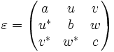
This allows your dielectric to have different dielectric constants for fields polarized in different directions. The epsilon tensor must be positive-definite (have all positive eigenvalues); if it is not, MPB exits with an error. (This does not imply that all of the entries of the epsilon matrix need be positive.) The components of the tensor are specified via three properties:
-
epsilon-diag[vector3] - The diagonal elements (a b c) of the dielectric tensor. No default value.
-
epsilon-offdiag[cvector3] - The off-diagonal elements (u v w) of the dielectric tensor. Defaults to zero. This is a
cvector3, which simply means that the components may be complex numbers (e.g.3+0.1i). If non-zero imaginary parts are specified, then the dielectric tensor is complex-hermitian. This is only supported when MPB is configured with the--with-hermitian-epsflag. This is not dissipative (the eigenvalues of epsilon are real), but rather breaks time-reversal symmetry, corresponding to a gyrotropic (magneto-optic) material (see our online textbook, ch. 2). Note that inversion symmetry may not mean what you expect for complex-hermitian epsilon, so be cautious about usingmpbiin this case. -
epsilon-offdiag-imag[vector3] - Deprecated: The imaginary parts of the off-diagonal elements (u v w) of the dielectric tensor; defaults to zero. Setting the imaginary parts directly by specifying complex numbers in
epsilon-offdiagis preferred.
-
For example, a material with a dielectric constant of 3.0 for TE fields (polarized in the xy plane) and 5.0 for TM fields (polarized in the z direction) would be specified via (make (dielectric-anisotropic (epsilon-diag 3 3 5))). Please be aware that not all 2d anisotropic dielectric structures will have TE and TM modes, however.
-
material-function - This material type allows you to specify the material as an arbitrary function of position. (For an example of this, see the
bragg-sine.ctlfile in theexamples/directory.) It has one property:-
material-func[function] - A function of one argument, the position
vector3(in lattice coordinates), that returns the material at that point. Note that the function you supply can return any material; wild and crazy users could even return anothermaterial-functionobject (which would then have its function invoked in turn). - Instead of
material-func, you can useepsilon-func: forepsilon-func, you give it a function of position that returns the dielectric constant at that point.
-
Normally, the dielectric constant is required to be positive (or positive-definite, for a tensor). However, MPB does have a somewhat experimental feature allowing negative dielectrics (e.g. in a plasma). To use it, call the function (allow-negative-epsilon) before (run). In this case, it will output the (real) frequency squared in place of the (possibly imaginary) frequencies. (Convergence will be somewhat slower because the eigenoperator is not positive definite.)
geometric-object
This class, and its descendants, are used to specify the solid geometric objects that form the dielectric structure being simulated. The base class is:
-
geometric-object - Properties:
-
material[material-typeclass] - The material that the object is made of (usually some sort of dielectric). No default value (must be specified).
-
center[vector3] - Center point of the object. No default value.
-
One normally does not create objects of type geometric-object directly, however; instead, you use one of the following subclasses. Recall that subclasses inherit the properties of their superclass, so these subclasses automatically have the material and center properties (which must be specified, since they have no default values).
Recall that all 3-vectors, including the center of an object, its axes, and so on, are specified in the basis of the normalized lattice vectors normalized to basis-size. Note also that 3-vector properties can be specified by either (property (vector3 x y z)) or, equivalently, (property x y z).
In a two-dimensional calculation, only the intersections of the objects with the x-y plane are considered.
-
sphere - A sphere. Properties:
-
radius[number] - Radius of the sphere. No default value.
-
-
cylinder - A cylinder, with circular cross-section and finite height. Properties:
-
radius[number] - Radius of the cylinder's cross-section. No default value.
-
height[number] - Length of the cylinder along its axis. No default value.
-
axis[vector3] - Direction of the cylinder's axis; the length of this vector is ignored. Defaults to point parallel to the z axis.
-
-
cone - A cone, or possibly a truncated cone. This is actually a subclass of
cylinder, and inherits all of the same properties, with one additional property. The radius of the base of the cone is given by theradiusproperty inherited fromcylinder, while the radius of the tip is given by the new property,radius2. (Thecenterof a cone is halfway between the two circular ends.)-
radius2[number] - Radius of the tip of the cone (i.e. the end of the cone pointed to by the
axisvector). Defaults to zero (a "sharp" cone).
-
-
block - A parallelepiped (i.e., a brick, possibly with non-orthogonal axes). Properties:
-
size[vector3] - The lengths of the block edges along each of its three axes. Not really a 3-vector (at least, not in the lattice basis), but it has three components, each of which should be nonzero. No default value.
-
e1,e2,e3[vector3] - The directions of the axes of the block; the lengths of these vectors are ignored. Must be linearly independent. They default to the three lattice directions.
-
-
ellipsoid - An ellipsoid. This is actually a subclass of
block, and inherits all the same properties, but defines an ellipsoid inscribed inside the block.
Here are some examples of geometric objects created using the above classes, assuming that the lattice directions (the basis) are just the ordinary unit axes, and m is some material we have defined:
; A cylinder of infinite radius and height 0.25 pointing along the x axis,
; centered at the origin:
(make cylinder (center 0 0 0) (material m)
               (radius infinity) (height 0.25) (axis 1 0 0))
; An ellipsoid with its long axis pointing along (1,1,1), centered on
; the origin (the other two axes are orthogonal and have equal
; semi-axis lengths):
(make ellipsoid (center 0 0 0) (material m)
                (size 0.8 0.2 0.2)
               (e1 1 1 1)
               (e2 0 1 -1)
               (e3 -2 1 1))
; A unit cube of material m with a spherical air hole of radius 0.2 at
; its center, the whole thing centered at (1,2,3):
(set! geometry (list
               (make block (center 1 2 3) (material m) (size 1 1 1))
               (make sphere (center 1 2 3) (material air) (radius 0.2))))
Functions
Here, we describe the functions that are defined by the Photonic-Bands package. There are many types of functions defined, ranging from utility functions for duplicating geometric objects to run functions that start the computation.
See also the reference section of the libctl manual, which describes a number of useful functions defined by libctl.
Geometry utilities
Some utility functions are provided to help you manipulate geometric objects:
-
(shift-geometric-object obj shift-vector) - Translate
objby the 3-vectorshift-vector. -
(geometric-object-duplicates shift-vector min-multiple max-multiple obj) - Return a list of duplicates of
obj, shifted by various multiples ofshift-vector(frommin-multipletomax-multiple, inclusive, in steps of 1). -
(geometric-objects-duplicates shift-vector min-multiple max-multiple obj-list) - Same as
geometric-object-duplicates, except operates on a list of objects,obj-list. If A appears before B in the input list, then all the duplicates of A appear before all the duplicates of B in the output list. -
(geometric-objects-lattice-duplicates obj-list [ ux uy uz ]) - Duplicates the objects in
obj-listby multiples of the lattice basis vectors, making all possible shifts of the "primitive cell" (see below) that fit inside the lattice cell. (This is useful for supercell calculations; see the [user-tutorial.html tutorial].) The primitive cell to duplicate isuxbyuybyuz, in units of the basis vectors. These three parameters are optional; any that you do not specify are assumed to be1. -
(point-in-object? point obj) - Returns whether or not the given 3-vector
pointis inside the geometric objectobj. -
(point-in-periodic-object? point obj) - As
point-in-object?, but also checks translations of the given object by the lattice vectors. -
(display-geometric-object-info indent-by obj) - Outputs some information about the given
obj, indented byindent-byspaces.
Coordinate conversion functions
The following functions allow you to easily convert back and forth between the lattice, cartesian, and reciprocal bases. (See also the note on units in the tutorial.)
-
(lattice->cartesian x),(cartesian->lattice x) - Convert
xbetween the lattice basis (the basis of the lattice vectors normalized tobasis-size) and the ordinary cartesian basis, wherexis either avector3or amatrix3x3, returning the transformed vector/matrix. In the case of a matrix argument, the matrix is treated as an operator on vectors in the given basis, and is transformed into the same operator on vectors in the new basis. -
(reciprocal->cartesian x),(cartesian->reciprocal x) - Like the above, except that they convert to/from reciprocal space (the basis of the reciprocal lattice vectors). Also, the cartesian vectors output/input are in units of 2π.
-
(reciprocal->lattice x),(lattice->reciprocal x) - Convert between the reciprocal and lattice bases, where the conversion again leaves out the factor of 2π (i.e. the lattice-basis vectors are assumed to be in units of 2π).
Also, a couple of rotation functions are defined, for convenience, so that you don't have to explicitly convert to cartesian coordinates in order to use libctl's rotate-vector3 function (see the Libctl User Reference):
-
(rotate-lattice-vector3 axis theta v),(rotate-reciprocal-vector3 axis theta v) - Like
rotate-vector3, except thataxisandvare specified in the lattice/reciprocal bases.
Usually, k-points are specified in the first Brillouin zone, but sometimes it is convenient to specify an arbitrary k-point. However, the accuracy of MPB degrades as you move farther from the first Brillouin zone (due to the choice of a fixed planewave set for a basis). This is easily fixed: simply transform the k-point to a corresponding point in the first Brillouin zone, and a completely equivalent solution (identical frequency, fields, etcetera) is obtained with maximum accuracy. The following function accomplishes this:
-
(first-brillouin-zone k) - Given a k-point
k(in the basis of the reciprocal lattice vectors, as usual), return an equivalent point in the first Brillouin zone of the current lattice (geometry-lattice).
Note that first-brillouin-zone can be applied to the entire k-points list with the Scheme expression: (map first-brillouin-zone k-points).
Run functions
These are functions to help you run and control the simulation. The ones you will most commonly use are the run function and its variants. The syntax of these functions, and one lower-level function, is:
-
(run band-func ...) - This runs the simulation described by the input parameters (see above), with no constraints on the polarization of the solution. That is, it reads the input parameters, initializes the simulation, and solves for the requested eigenstates of each k-point. The dielectric function is outputted to "
epsilon.h5" before any eigenstates are computed.runtakes as arguments zero or more "band functions"band-func. A band function should be a function of one integer argument, the band index, so that(band-func which-band)performs some operation on the bandwhich-band(e.g. outputting fields). After every k-point, each band function is called for the indices of all the bands that were computed. Alternatively, a band function may be a "thunk" (function of zero arguments), in which case(band-func)is called exactly once per k-point. -
(run-zeven band-func ...), (run-zodd band-func ...) - These are the same as the
runfunction except that they constrain their solutions to have even and odd symmetry with respect to the z=0 plane. You should use these functions only for structures that are symmetric through the z=0 mirror plane, where the third basis vector is in the z direction (0,0,1) and is orthogonal to the other two basis vectors, and when the k vectors are in the xy plane. Under these conditions, the eigenmodes always have either even or odd symmetry. In two dimensions, even/odd parities are equivalent to TE/TM polarizations, respectively (and are often strongly analogous even in 3d). Such a symmetry classification is useful for structures such as waveguides and photonic-crystal slabs. (For example, see the paper by S. G. Johnson et al., "Guided modes in photonic crystal slabs," PRB 60, 5751, August 1999.) -
(run-te band-func ...), (run-tm band-func ...) - These are the same as the
runfunction except that they constrain their solutions to be TE- and TM-polarized, respectively, in two dimensions. The TE and TM polarizations are defined has having electric and magnetic fields in the xy plane, respectively. Equivalently, the H/E field of TE/TM light has only a z component (making it easier to visualize).
These functions are actually equivalent to calling run-zeven and run-zodd, respectively.
Note that for the modes to be segregated into TE and TM polarizations, the dielectric function must have mirror symmetry for reflections through the xy plane. If you use anisotropic dielectrics, you should be aware that they break this symmetry if the z direction is not one of the principle axes. If you use run-te or run-tm in such a case of broken symmetry, MPB will exit with an error.
-
(run-yeven band-func ...), (run-yodd band-func ...) - These functions are analogous to
run-zevenandrun-zodd, except that they constrain their solutions to have even and odd symmetry with respect to the y=0 plane. You should use these functions only for structures that are symmetric through the y=0 mirror plane, where the second basis vector is in the y direction (0,1,0) and is orthogonal to the other two basis vectors, and when the k vectors are in the xz plane. -
run-yeven-zeven,run-yeven-zodd,run-yodd-zeven,run-yodd-zodd,run-te-yeven,run-te-yodd,run-tm-yeven,run-tm-yodd - These
run-like functions combine theyeven/yoddconstraints withzeven/zoddorte/tm. See alsorun-parity, below. -
(run-parity p reset-fields band-func ...) - Like the
runfunction, except that it takes two extra parameters, a paritypand a boolean (true/false) valuereset-fields.pspecifies a parity constraint, and should be one of the predefined variables:-
NO-PARITY: equivalent torun -
EVEN-Z(orTE): equivalent torun-zevenorrun-te -
ODD-Z(orTM): equivalent torun-zoddorrun-tm -
EVEN-Y(likeEVEN-Zbut for y=0 plane) -
ODD-Y(likeODD-Zbut for y=0 plane)
-
It is possible to specify more than one symmetry constraint simultaneously by adding them, e.g. (+ EVEN-Z ODD-Y) requires the fields to be even through z=0 and odd through y=0. It is an error to specify incompatible constraints (e.g. (+ EVEN-Z ODD-Z)). Important: if you specify the z/y parity, the dielectric structure (and the k vector) must be symmetric about the z/y=0 plane, respectively.
If reset-fields is false, the fields from any previous calculation will be reused as the starting point from this calculation, if possible; otherwise, the fields are reset to random values. The ordinary run functions use a default reset-fields oftrue. Alternatively, reset-fields may be a string, the name of an HDF5 file to load the initial fields from (as exported by save-eigenvectors, below).
-
(display-eigensolver-stats) - Display some statistics on the eigensolver convergence; this function is useful mainly for MPB developers in tuning the eigensolver.
Several band functions for outputting the eigenfields are defined for your convenience, and are described in the Band output functions section, below. You can also define your own band functions, and for this purpose the functions described in the section Field manipulation functions, below, are useful. A band function takes the form:
(define (my-band-func which-band)
  ...do stuff here with band index which-band...
)
Note that the output variable freqs may be used to retrieve the frequency of the band (see above). Also, a global variable current-k is defined holding the current k-point vector from the k-points list.
There are also some even lower-level functions that you can call, although you should not need to do most of the time:
-
(init-params p reset-fields?) - Read the input variables and initialize the simulation in preparation for computing the eigenvalues. The parameters are the same as the first two parameters of
run-parity. This function must be called before any of the other simulation functions below. (Note, however, that therunfunctions all callinit-params.) -
(set-parity p) - After calling
init-params, you can change the parity constraint without resetting the other parameters by calling this function. Beware that this does not randomize the fields (see below); you don't want to try to solve for, say, the TM eigenstates when the fields are initialized to TE states from a previous calculation. -
(randomize-fields) - Initialize the fields to random values.
-
(solve-kpoint k) - Solve for the requested eigenstates at the Bloch wavevector
k.
The inverse problem: k as a function of frequency
MPB's (run) function(s) and its underlying algorithms compute the frequency w as a function of wavevector k. Sometimes, however, it is desirable to solve the inverse problem, for k at a given frequency w. This is useful, for example, when studying coupling in a waveguide between different bands at the same frequency (frequency is conserved even when wavevector is not). One also uses k(w) to construct wavevector diagrams, which aid in understanding diffraction (e.g. negative-diffraction materials and super-prisms). To solve such problems, therefore, we provide the find-k function described below, which inverts w(k) via a few iterations of Newton's method (using the group velocity dw/dk). Because it employs a root-finding method, you need to specify bounds on k and a crude initial guess (order of magnitude is usually good enough).
-
(find-k p omega band-min band-max kdir tol kmag-guess kmag-min kmag-max [band-func...]) - Find the wavevectors in the current geometry/structure for the bands from
band-mintoband-maxat the frequencyomegaalong thekdirdirection in k-space. Returns a list of the wavevector magnitudes for each band; the actual wavevectors are(vector3-scale magnitude (unit-vector3 kdir)). The arguments offind-kare:-
p: parity (same as first argument torun-parity, above). -
omega: the frequency at which to find the bands -
band-min,band-max: the range of bands to solve for the wavevectors of (inclusive). -
kdir: the direction in k-space in which to find the wavevectors. (The magnitude ofkdiris ignored.) -
tol: the fractional tolerance with which to solve for the wavevector;1e-4is usually sufficient. (Like thetoleranceinput variable, this is only the tolerance of the numerical iteration...it does not have anything to do with e.g. the error from finite gridresolution.) -
kmag-guess: an initial guess for the k magnitude (alongkdir) of the wavevector atomega. Can either be a list (one guess for each band fromband-mintoband-max) or a single number (same guess for all bands, which is usually sufficient). -
kmag-min,kmag-max: a range of k magnitudes to search; should be large enough to include the correct k values for all bands. -
band-func: zero or more band functions, just as in(run), which are evaluated at the computed k points for each band.
-
The find-k routine also prints a line suitable for grepping:
kvals: omega, band-min, band-max, kdir1, kdir2, kdir3, k magnitudes...
Band/output functions
All of these are functions that, given a band index, output the corresponding field or compute some function thereof (in the primitive cell of the lattice). They are designed to be passed as band functions to the run routines, although they can also be called directly. See also the section on field normalizations.
-
(output-hfield which-band) -
(output-hfield-x which-band) -
(output-hfield-y which-band) -
(output-hfield-z which-band) - Output the magnetic (H) field for
which-band; either all or one of the (Cartesian) components, respectively. -
(output-dfield which-band) -
(output-dfield-x which-band) -
(output-dfield-y which-band) -
(output-dfield-z which-band) - Output the electric displacement (D) field for
which-band; either all or one of the (Cartesian) components, respectively. -
(output-efield which-band) -
(output-efield-x which-band) -
(output-efield-y which-band) -
(output-efield-z which-band) - Output the electric (E) field for
which-band; either all or one of the (Cartesian) components, respectively. -
(output-hpwr which-band) - Output the time-averaged magnetic-field energy density (hpwr =
 for
for which-band. -
(output-dpwr which-band) - Output the time-averaged electric-field energy density (dpwr =
 ) for
) for which-band. -
(fix-hfield-phase which-band) -
(fix-dfield-phase which-band) -
(fix-efield-phase which-band) - Fix the phase of the given eigenstate in a canonical way based on the given spatial field (see also
fix-field-phase, below). Otherwise, the phase is random; these functions also maximize the real part of the given field so that one can hopefully just visualize the real part. To fix the phase for output, pass one of these functions torunbefore the corresponding output function, e.g.(run-tm fix-dfield-phase output-dfield-z)
Although we try to maximize the "real-ness" of the field, this has a couple of limitations. First, the phase of the different field components cannot, of course, be chosen independently, so an individual field component may still be imaginary. Second, if you use mpbi to take advantage of inversion symmetry in your problem, the phase is mostly determined elsewhere in the program; fix-_field-phase in that case only determines the sign.
See also below for the output-poynting and output-tot-pwr functions to output the Poynting vector and the total electromagnetic energy density, respectively, and the output-charge-density function to output the bound charge density.
Sometimes, you only want to output certain bands. For example, here is a function that, given an band/output function like the ones above, returns a new output function that only calls the first function for bands with a large fraction of their energy in an object(s). (This is useful for picking out defect states in supercell calculations.)
-
(output-dpwr-in-objects band-func min-energy objects...) - Given a band function
band-func, returns a new band function that only callsband-funcfor bands having a fraction of their electric-field energy greater thanmin-energyinside the given objects (zero or more geometric objects). Also, for each band, prints the fraction of their energy in the objects in the following form (suitable for grepping):
dpwr:, band-index, frequency, energy-in-objects
output-dpwr-in-objects only takes a single band function as a parameter, but if you want it to call several band functions, you can easily combine them into one with the following routine:
-
(combine-band-functions band-funcs...) - Given zero or more band functions, returns a new band function that calls all of them in sequence. (When passed zero parameters, returns a band function that does nothing.)
It is also often useful to output the fields only at a certain k-point, to let you look at typical field patterns for a given band while avoiding gratuitous numbers of output files. This can be accomplished via:
-
(output-at-kpoint k-point band-funcs...) - Given zero or more band functions, returns a new band function that calls all of them in sequence, but only at the specified
k-point. For other k-points, does nothing.
Miscellaneous functions
-
(retrieve-gap lower-band) - Return the frequency gap from the band #
lower-bandto the band #(lower-band+1), as a percentage of mid-gap frequency. The "gap" may be negative if the maximum of the lower band is higher than the minimum of the upper band. (The gap is computed from theband-range-dataof the previous run.)
Parity
Given a set of eigenstates at a k-point, MPB can compute their parities with respect to the z=0 or y=0 plane. The z/y parity of a state is defined as the expectation value (under the usual inner product) of the mirror-flip operation through z/y=0, respectively. For true even and odd eigenstates (see e.g. run-zeven and run-zodd), this will be +1 and -1, respectively; for other states it will be something in between.
This is useful e.g. when you have a nearly symmetric structure, such as a waveguide with a substrate underneath, and you want to tell which bands are even-like (parity > 0) and odd-like (parity < 0). Indeed, any state can be decomposed into purely even and odd functions, with absolute-value-squared amplitudes of (1+parity)/2 and (1-parity)/2, respectively.
-
display-zparities,display-yparities - These are band functions, designed to be passed to
(run), which output all of the z/y parities, respectively, at each k-point (in comma-delimited format suitable for grepping). -
(compute-zparities) - Returns a list of the parities about the z=0 plane, one number for each band computed at the last k-point.
-
(compute-yparities) - Returns a list of the parities about the y=0 plane, one number for each band computed at the last k-point.
(The reader should recall that the magnetic field is only a pseudo-vector, and is therefore multiplied by -1 under mirror-flip operations. For this reason, the magnetic field appears to have opposite symmetry from the electric field, but is really the same.)
Group velocities
Given a set of eigenstates at a given k-point, MPB can compute their group velocities (the derivative  of frequency with respect to wavevector) using the Hellman-Feynmann theorem. Three functions are provided for this purpose, and we document them here from highest-level to lowest-level.
-
display-group-velocities - This is a band function, designed to be passed to
(run), which outputs all of the group velocity vectors (in the Cartesian basis, in units of c) at each k-point. -
(compute-group-velocities) - Returns a list of group-velocity vectors (in the Cartesian basis, units of c) for the bands at the last-computed k-point.
-
(compute-group-velocity-component direction) - Returns a list of the group-velocity components (units of c) in the given direction, one for each band at the last-computed k-point. direction is a vector in the reciprocal-lattice basis (like the k-points); its length is ignored. (This has the advantage of being three times faster than
compute-group-velocities.) -
(compute-1-group-velocity which-band),(compute-1-group-velocity-component direction which-band) - As above, but returns the group velocity or component thereof only for band
which-band.
Field manipulation
The Photonic-Bands package provides a number of ways to take the field of a band and manipulate, process, or output it. These methods usually work in two stages. First, one loads a field into memory (computing it in position space) by calling one of the get functions below. Then, other functions can be called to transform or manipulate the field.
The simplest class of operations involve only the currently-loaded field, which we describe in the second subsection below. To perform more sophisticated operations, involving more than one field, one must copy or transform the current field into a new field variable, and then call one of the functions that operate on multiple field variables (described in the third subsection).
Field normalization
In order to perform useful operations on the fields, it is important to understand how they are normalized. We normalize the fields in the way that is most convenient for perturbation and coupled-mode theory [c.f. SGJ et al., PRE 65, 066611 (2002)] (see also our online textbook, ch. 2), so that their energy densities have unit integral. In particular, we normalize the electric ( ), displacement (
 ) and magnetic (
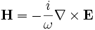 ) fields, so that:
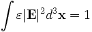
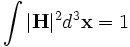
where the integrals are over the computational cell. Note the volume element  (the volume of a grid pixel/voxel). If you simply sum over all the grid points, therefore, you will get (# grid points) / (volume of cell).
Note that we have dropped the pesky factors of 1/2, π, etcetera from the energy densities, since these do not appear in e.g. perturbation theory, and the fields have arbitrary units anyway. The functions to compute/output energy densities below similarly use and without any prefactors.
Loading and manipulating the current field
In order to load a field into memory, call one of the get functions follow. They should only be called after the eigensolver has run (or after init-params, in the case of get-epsilon). One normally calls them after run, or in one of the band functions passed to run.
-
(get-hfield which-band) - Loads the magnetic (H) field for the band
which-band. -
(get-dfield which-band) - Loads the electric displacement (D) field for the band
which-band. -
(get-efield which-band) - Loads the electric (E) field for the band
which-band. (This function actually callsget-dfieldfollowed byget-efield-from-dfield, below.) -
(get-charge-density which-band) - Loads the bound charge density
 for the band
 which-band. -
(get-epsilon) - Loads the dielectric function.
Once loaded, the field can be transformed into another field or a scalar field:
-
(get-efield-from-dfield) - Multiplies by the inverse dielectric tensor to compute the electric field from the displacement field. Only works if a D field has been loaded.
-
(fix-field-phase) - Fix the currently-loaded eigenstate's phase (which is normally random) in a canonical way, based on the spatial field (H, D, or E) that has currently been loaded. The phase is fixed to make the real part of the spatial field as big as possible (so that you can hopefully visualize just the real part of the field), and a canonical sign is chosen. See also the
fix-*field-phaseband functions, above, which are convenient wrappers aroundfix-field-phase -
(compute-field-energy) - Given the H or D fields, computes the corresponding energy density function (normalized by the total energy in H or D, respectively). Also prints the fraction of the field in each of its cartesian components in the following form (suitable for grepping):
f-energy-components:, k-index, band-index, x-fraction, y-fraction, z-fraction
where f is either h or d. The return value of compute-field-energy is a list of 7 numbers: (U xr xi yr yi zr zi). U is the total, unnormalized energy, which is in arbitrary units deriving from the normalization of the eigenstate (e.g. the total energy for H is always 1.0). xr is the fraction of the energy in the real part of the field's x component, xi is the fraction in the imaginary part of the x component, etcetera (yr + yi = y-fraction, and so on).
-
(compute-field-divergence) - Given a vector field, compute its divergence.
Various integrals and other information about the eigenstate can be accessed by the following functions, useful e.g. for perturbation theory. Functions dealing with the field vectors require a field to be loaded, and functions dealing with the energy density require an energy density to be loaded via compute-field-energy.
-
(compute-energy-in-dielectric min-eps max-eps) - Returns the fraction of the energy that resides in dielectrics with epsilon in the range
min-epstomax-eps. -
(compute-energy-in-objects objects...) - Returns the fraction of the energy inside zero or more geometric objects.
-
(compute-energy-integral f) -
fis a function(f u eps r)that returns a number given three parameters:u, the energy density at a point;eps, the dielectric constant at the same point; andr, the position vector (in lattice coordinates) of the point.compute-energy-integralreturns the integral offover the unit cell. (The integral is computed simply as the sum over the grid points times the volume of a grid pixel/voxel.) This can be useful e.g. for perturbation-theory calculations. -
(compute-field-integral f) - Like
compute-energy-integral, butfis a function(f F eps r)that returns a number (possibly complex) whereFis the complex field vector at the given point. -
(get-epsilon-point r) - Given a position vector
r(in lattice coordinates), return the interpolated dielectric constant at that point. (Since MPB uses a an effective dielectric tensor internally, this actually returns the mean dielectric constant.) -
(get-epsilon-inverse-tensor-point r) - Given a position vector
r(in lattice coordinates), return the interpolated inverse dielectric tensor (a 3x3 matrix) at that point. (Near a dielectric interface, the effective dielectric constant is a tensor even if you input only scalar dielectrics; see the epsilon overview for more information.) The returned matrix may be complex-Hermetian if you are employing magnetic materials. -
(get-energy-point r) - Given a position vector
r(in lattice coordinates), return the interpolated energy density at that point. -
(get-field-point r) - Given a position vector
r(in lattice coordinates), return the interpolated (complex) field vector at that point. -
(get-bloch-field-point r) - Given a position vector
r(in lattice coordinates), return the interpolated (complex) Bloch field vector at that point (this is the field without the exp(ikx) envelope).
Finally, we have the following functions to output fields (either the vector fields, the scalar energy density, or epsilon), with the option of outputting several periods of the lattice.
-
(output-field [ nx [ ny [ nz ] ] ]) -
(output-field-x [ nx [ ny [ nz ] ] ]) -
(output-field-y [ nx [ ny [ nz ] ] ]) -
(output-field-z [ nx [ ny [ nz ] ] ]) - Output the currently-loaded field. The optional (as indicated by the brackets) parameters
nx,ny, andnzindicate the number of periods to be outputted along each of the three lattice directions. Omitted parameters are assumed to be 1. For vector fields,output-fieldoutputs all of the (Cartesian) components, while the other variants output only one component. -
(output-epsilon [ nx [ ny [ nz ] ] ]) - A shortcut for calling
get-epsilonfollowed byoutput-field. Note that, because epsilon is a tensor, a number of datasets are outputted in"epsilon.h5":-
"data": 3/trace(1/epsilon) -
"epsilon.{xx,xy,xz,yy,yz,zz}": the (Cartesian) components of the (symmetric) dielectric tensor. -
"epsilon_inverse.{xx,xy,xz,yy,yz,zz}": the (Cartesian) components of the (symmetric) inverse dielectric tensor.
-
Storing and combining multiple fields
In order to perform operations involving multiple fields, e.g. computing the Poynting vector  , they must be stored in field variables. Field variables come in three flavors, real-scalar (rscalar) fields, complex-scalar (cscalar) fields, and complex-vector (cvector) fields. There is a pre-defined field variable
 cur-field representing the currently-loaded field (see above), and you can "clone" it to create more field variables with one of:
-
(field-make f) - Return a new field variable of the same type and size as the field variable
f. Does not copy the field contents (seefield-copyandfield-set!, below). -
(rscalar-field-make f) -
(cscalar-field-make f) -
(cvector-field-make f) - Like
field-make, but return a real-scalar, complex-scalar, or complex-vector field variable, respectively, of the same size asfbut ignoringf's type. -
(cvector-field-nonbloch! f) - By default, complex vector fields are assumed to be Bloch-periodic (and are multiplied by eikx in output routines). This function tells MPB that the complex vector field f should never be multiplied by Bloch phases.
-
(field-set! fdest fsrc) - Set
fdestto store the same field values asfsrc, which must be of the same size and type. -
(field-copy f) - Return a new field variable that is exact copy of
f; this is equivalent to callingfield-makefollowed byfield-set!. -
(field-load f) - Loads the field
fas the current field, at which point you can use all of the functions in the previous section to operate on it or output it.
Once you have stored the fields in variables, you probably want to compute something with them. This can be done in three ways: combining fields into new fields with field-map! (e.g. combine E and H to ), integrating some function of the fields with integrate-fields (e.g. to compute coupling integrals for perturbation theory), and getting the field values at arbitrary points with *-field-get-point (e.g. to do a line or surface integral). These three functions are described below:
-
(field-map! fdest func [f1 f2 ...]) - Compute the new field
fdestto be(func f1-val f2-val ...)at each point in the grid, wheref1-valetcetera is the corresponding value off1etcetera. All the fields must be of the same size, and the argument and return types offuncmust match those of thef1...andfdestfields, respectively.fdestmay be the same field as one of thef1...arguments. Note: all fields are without Bloch phase factors exp(ikx). -
(integrate-fields func [f1 f2 ...]) - Compute the integral of the function
(func r [f1 f2 ...])over the computational cell, whereris the position (in the usual lattice basis) andf1etc. are fields (which must all be of the same size). (The integral is computed simply as the sum over the grid points times the volume of a grid pixel/voxel.) Note: all fields are without Bloch phase factors exp(ikx). See also the note below. -
(cvector-field-get-point f r) -
(cvector-field-get-point-bloch f r) -
(rscalar-field-get-point f r) - Given a position vector
r(in lattice coordinates), return the interpolated field cvector/rscalar fromfat that point.cvector-field-get-point-blochreturns the field without the exp(ikx) Bloch wavevector, in analogue toget-bloch-field-point.
You may be wondering how to get rid of the field variables once you are done with them: you don't, since they are garbage collected automatically.
We also provide functions, in analogue to e.g get-efield and output-efield above, to "get" various useful functions as the current field and to output them to a file:
-
(get-poynting which-band) - Loads the Poynting vector for the band
which-band, the flux density of electromagnetic energy flow, as the current field. 1/2 of the real part of this vector is the time-average flux density (which can be combined with the imaginary part to determine the amplitude and phase of the time-dependent flux). -
(output-poynting which-band) -
(output-poynting-x which-band) -
(output-poynting-y which-band) -
(output-poynting-z which-band) - Output the Poynting vector field for
which-band; either all or one of the (Cartesian) components, respectively. -
(get-tot-pwr which-band) - Load the time-averaged electromagnetic-field energy density (
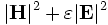 ) for
) for which-band. (If you multiply the real part of the Poynting vector by a factor of 1/2, above, you should multiply by a factor of 1/4 here for consistency.) -
(output-tot-pwr which-band) - Output the time-averaged electromagnetic-field energy density (above) for
which-band. -
(output-charge-density which-band) - Output the bound charge density (above) for
which-band.
As an example, below is the Scheme source code for the get-poynting function, illustrating the use of the various field functions:
(define (get-poynting which-band)
  (get-efield which-band)                      ; put E in cur-field
  (let ((e (field-copy cur-field)))            ; ... and copy to local var.
    (get-hfield which-band)                    ; put H in cur-field
    (field-map! cur-field                      ; write ExH to cur-field
                (lambda (e h) (vector3-cross (vector3-conj e) h))
                e cur-field)
    (cvector-field-nonbloch! cur-field)))      ; see below
Stored fields and Bloch phases
Complex vector fields like E and H as computed by MPB are physically of the Bloch form: exp(ikx) times a periodic function. What MPB actually stores, however, is just the periodic function, the Bloch envelope, and only multiplies by exp(ikx) for when the fields are output or passed to the user (e.g. in integration functions). This is mostly transparent, with a few exceptions noted above for functions that do not include the exp(ikx) Bloch phase (it is somewhat faster to operate without including the phase).
On some occasions, however, when you create a field with field-map!, the resulting field should not have any Bloch phase. For example, for the Poynting vector E*xH, the exp(ikx) cancels because of the complex conjugation. After creating this sort of field, we must use the special function cvector-field-nonbloch! to tell MPB that the field is purely periodic:
-
(cvector-field-nonbloch! f) - Specify that the field
fis not of the Bloch form, but rather that it is purely periodic.
Currently, all fields must be either Bloch or non-Bloch (i.e. periodic), which covers most physically meaningful possibilities.
There is another wrinkle: even for fields in Bloch form, the exp(ikx) phase currently always uses the current k-point, even if the field was computed from another k-point. So, if you are performing computations combining fields from different k-points, you should take care to always use the periodic envelope of the field, putting the Bloch phase in manually if necessary.
Manipulating the raw eigenvectors
MPB also includes a few low-level routines to manipulate the raw eigenvectors that it computes in a transverse planewave basis.
The most basic operations involve copying, saving, and restoring the current set of eigenvectors or some subset thereof:
-
(get-eigenvectors first-band num-bands) - Return an eigenvector object that is a copy of
num-bandscurrent eigenvectors starting atfirst-band. e.g. to get a copy of all of the eigenvectors, use(get-eigenvectors 1 num-bands). -
(set-eigenvectors ev first-band) - Set the current eigenvectors, starting at
first-band, to those in theeveigenvector object (as returned byget-eigenvectors). (Does not work if the grid sizes don't match) -
(load-eigenvectors filename) -
(save-eigenvectors filename) - Read/write the current eigenvectors (raw planewave amplitudes) to/from an HDF5 file named
filename. Instead of usingload-eigenvectorsdirectly, you can pass thefilenameas thereset-fieldsparameter ofrun-parity, above. (Loaded eigenvectors must be of the same size (same grid size and #bands) as the current settings.)
Currently, there's only one other interesting thing you can do with the raw eigenvectors, and that is to compute the dot-product matrix between a set of saved eigenvectors and the current eigenvectors. This can be used, e.g., to detect band crossings or to set phases consistently at different k points. The dot product is returned as a "sqmatrix" object, whose elements can be read with the sqmatrix-size and sqmatrix-ref routines.
-
(dot-eigenvectors ev first-band) - Returns a sqmatrix object containing the dot product of the saved eigenvectors
evwith the current eigenvectors, starting atfirst-band. That is, the (i,j)th output matrix element contains the dot product of the (i+1)th vector ofev(conjugated) with the (first-band+j)th eigenvector. Note that the eigenvectors, when computed, are orthonormal, so the dot product of the eigenvectors with themselves is the identity matrix. -
(sqmatrix-size sm) - Return the size n of an nxn sqmatrix
sm. -
(sqmatrix-ref sm i j) - Return the (
i,j)th element of the nxn sqmatrixsm, where {i,j} range from 0..n-1.
Inversion Symmetry
If you configure MPB with the --with-inv-symmetry flag, then the program is configured to assume inversion symmetry in the dielectric function. This allows it to run at least twice as fast and use half as much memory as the more general case. This version of MPB is by default installed as mpbi, so that it can coexist with the usual mpb program.
Inversion symmetry means that if you transform (x,y,z) to (-x,-y,-z) in the coordinate system, the dielectric structure is not affected. Or, more technically, that (see our online textbook, ch. 3):
where the conjugation is significant for complex-hermitian dielectric tensors. This symmetry is very common; all of the examples in this manual have inversion symmetry, for example.
Note that inversion symmetry is defined with respect to a specific origin, so that you may "break" the symmetry if you define a given structure in the wrong way—this will prevent mpbi from working properly. For example, the diamond structure that we considered earlier would not have possessed inversion symmetry had we positioned one of the "atoms" to lie at the origin.
You might wonder what happens if you pass a structure lacking inversion symmetry to mpbi. As it turns out, mpbi only looks at half of the structure, and infers the other half by the inversion symmetry, so the resulting structure always has inversion symmetry, even if its original description did not. So, you should be careful, and look at the epsilon.h5 output to make sure it is what you expected.
Parallel MPB
We provide two methods by which you can parallelize MPB. The first, using MPI, is the most sophisticated and potentially provides the greatest and most general benefits. The second, which involves a simple script to split e.g. the k-points list among several processes, is less general but may be useful in many cases.
MPB with MPI parallelization
If you configure MPB with the --with-mpi flag, then the program is compiled to take advantage of distributed-memory parallel machines with MPI, and is installed as mpb-mpi. (See also the installation section.) This means that computations will (potentially) run more quickly and take up less memory per processor than for the serial code. (Normally, you should also install the serial version of MPB, if only to get the mpb-data program, which is not installed with mpb-mpi.)
Using the parallel MPB is almost identical to using the serial version(s), with a couple of minor exceptions. The same ctl files should work for both. Running a program that uses MPI requires slightly different invocations on different systems, but will typically be something like:
unix% mpirun -np 4 mpb-mpi foo.ctl
to run on e.g. 4 processors. A second difference is that 1D systems are currently not supported in the MPI code, but the serial code should be fast enough for those anyway. A third difference is that the output HDF5 files (epsilon, fields, etcetera) from mpb-mpi have their first two dimensions (x and y) transposed; i.e. they are output as YxXxZ arrays. This doesn't prevent you from visualizing them, but the coordinate system is left-handed; to un-transpose the data, you can process it with mpb-data and the -T option (in addition to any other options).
In order to get optimal benefit (time and memory savings) from mpb-mpi, the first two dimensions (nx and ny) of your grid should both be divisible by the number of processes. If you violate this constraint, MPB will still work, but the load balance between processors will be uneven. At worst, e.g. if either nx or ny is smaller than the number of processes, then some of the processors will be idle for part (or all) of the computation. When using inversion symmetry (mpbi-mpi) for 2D grids only, the optimal case is somewhat more complicated: nx and (ny/2 + 1), not ny, should both be divisible by the number of processes.
mpb-mpi divides each band at each k-point between the available processors. This means that, even if you have only a single k-point (e.g. in a defect calculation) and/or a single band, it can benefit from parallelization. Moreover, memory usage per processor is inversely proportional to the number of processors used. For sufficiently large problems, the speedup is also nearly linear.
MPI support in MPB is thanks to generous support from Clarendon Photonics.
Alternative parallelization: mpb-split
There is an alternative method of parallelization when you have multiple k points: do each k-point on a different processor. This does not provide any memory benefits, and does not allow one k-point to benefit by starting with the fields of the previous k-point, but is easy and may be the only effective way to parallelize calculations for small problems. This method also does not require MPI: it can utilize the unmodified serial mpb program. To make it even easier, we supply a simple script called mpb-split (or mpbi-split) to break the k-points list into chunks for you. Running:
unix% mpb-split num-split foo.ctl
will break the k-points list in foo.ctl into num-split more-or-less equal chunks, launch num-split processes of mpb in parallel to process each chunk, and output the results of each in order. (Each process is an ordinary mpb execution, except that it numbers its k-points depending upon which chunk it is in, so that output files will not overwrite one another and you can still grep for frequencies as usual.)
Of course, this will only benefit you on a system where different processes will run on different processors, such as an SMP or a cluster with automatic process migration (e.g. MOSIX). mpb-split is actually a trivial shell script, though, so you can easily modify it if you need to use a special command to launch processes on other processors/machines (e.g. via GNU Queue).
The general syntax for mpb-split is:
unix% mpb-split num-split mpb-arguments...
where all of the arguments following num-split are passed along to mpb. What mpb-split technically does is to set the MPB variable k-split-num to num-split and k-split-index to the index (starting with 0) of the chunk for each process. If you want, you can use these variables to divide the problem in some other way and then reset them to 1 and , respectively.
Developer Information
| |
| MIT Photonic Bands |
| Download |
| Release notes |
| MPB manual |
| Introduction |
| Installation |
| User Tutorial |
| Data Analysis Tutorial |
| User Reference |
| Developer Information |
| Acknowledgements |
| License and Copyright |
Here, we begin with a brief overview of what the program is computing, and then describe how the program and computation are broken up into different portions of the code.
(A Chinese version of this document is also available.)
The Mathematics of MPB
This section provides a whirlwind tour of the mathematics of photonic band structure calculations and the algorithms that we employ. For more detailed information, see:
- Photonic Crystals: Molding the Flow of Light, by J. D. Joannopoulos, R. D. Meade, and J. N. Winn (Princeton, 1995).
- Steven G. Johnson and J. D. Joannopoulos, "Block-iterative frequency-domain methods for Maxwell's equations in a planewave basis," Optics Express 8, no. 3, 173-190 (2001).
The MIT Photonic-Bands Package takes a periodic dielectric structure and computes the eigenmodes of that structure, which are the electromagnetic waves that can propagate through the structure with a definite frequency. This corresponds to solving an eigenvalue problem
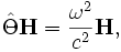
where  is the magnetic field, ω is the frequency, and
  is the Maxwell operator
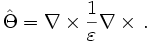
We also have an additional constraint, that  be zero (the magnetic field must be "transverse").
Since the structure is periodic, we can also invoke Bloch's theorem to write the states in the form:
where where  is a periodic function (the Bloch envelope) and
  is the Bloch wavevector. So, at each k-point (Bloch wavevector), we need to solve for a discrete set of eigenstates, the photonic bands of the structure.
To solve for the eigenstates on a computer, we must expand the magnetic field in some basis, where we truncate the basis to some finite number of points to discretize the problem. For example, we could use a traditional finite-element basis in which the field is taken on a finite number of mesh points and linearly interpolated in between. However, it is expensive to enforce the transversality constraint in this basis. Instead, we use a Fourier (spectral) basis, expanding the periodic part of the field as a sum of planewaves:
In this basis, the transversality constraint is easy to maintain, as it merely implies that the planewave amplitudes  must be orthogonal to
  .
.
In order to find the eigenfunctions, we could compute the elements of explicitly in our basis, and then call LAPACK or some similar code to find the eigenvectors and eigenvalues. For a three-dimensional calculation, this could mean finding the eigenvectors of a matrix with hundreds of thousands of elements on a side--daunting merely to store, much less compute. Fortunately, we only want to know a few eigenvectors, not hundreds of thousands, so we can use much less expensive iterative methods that don't require us to store explicitly.
Iterative eigensolvers require only that one supply a routine to operate on a vector (function). Starting with an initial guess for the eigenvector, they then converge quickly to the actual eigenvector, stopping when the desired tolerance is achieved. There are many iterative eigensolver methods; we use a preconditioned block minimization of the Rayleigh quotient which is further described in the file src/matrices/eigensolver.c. In the Fourier basis, applying to a function is relatively easy: the curls become cross products with  ; the multiplication by
  is performed by using an FFT to transform to the spatial domain, multiplying, and then transforming back with an inverse FFT. For more information and references on iterative eigensolvers, see the paper cited above.
We also support a "targeted" eigensolver. A typical iterative eigensolver finds the p lowest eigenvalues and eigenvectors. Instead, we can find the p eigenvalues closest to a given frequency ω0 by solving for the eigenvalues of  instead of . This new operator has the same eigenvectors as , but its eigenvalues have been shifted to make those closest to ω0 the smallest. (This is not really the best algorithm to find interior eigenvalues like this; a future version of MPB may use ARPACK-style shift-and-invert Arnoldi, or perhaps the Jacobi-Davidson algorithm.)
The eigensolver we use is preconditioned, which means that convergence can be greatly improved by suppling a good preconditioner matrix. Finding a good preconditioner involves making an approximate inverse of , and is something of a black art with lots of trial and error.
Dielectric Function Computation
The initialization of the dielectric function deserves some additional discussion, both because it is crucial for good convergence, and because we use somewhat complicated algorithms for performance reasons.
To ameliorate the convergence problems caused in a planewave basis by a discontinuous dielectric function, the dielectric function is smoothed (averaged) at the resolution of the grid. Another way of thinking about it is that this brings the average dielectric constant (over the grid) closer to its true value. Since different polarizations of the field prefer different averaging methods, one has to construct an effective dielectric tensor at the boundaries between dielectrics, as described by the paper referenced above.
This averaging has two components. First, at each grid point the dielectric constant (epsilon) and its inverse are averaged over a uniform mesh extending halfway to the neighboring grid points. (The mesh resolution is controlled by the mesh-size user input variable.) Second, for grid points on the boundary between two dielectrics, we compute the vector normal to the dielectric interface; this is done by averaging the "dipole moment" of the dielectric function over a spherically-symmetric distribution of points. The normal vector and the two averages of epsilon are then combined into an effective dielectric tensor for the grid point.
All of this averaging is handled by a subroutine in src/maxwell/ (see below) that takes as input a function epsilon(r), which returns the dielectric constant for a given position r. This epsilon function must be as efficient as possible, because it is evaluated a large number of times: the size of the grid multiplied by mesh-size3 (in three dimensions).
To specify the geometry, the user provides a list of geometric objects (blocks, spheres, cylinders and so on). These are parsed into an efficient data structure and are used to to provide the epsilon function described above. (All of this is handled by the libctlgeom component of libctl, described below.) At the heart of the epsilon function is a routine to return the geometric object enclosing a given point, taking into account the fact that the objects are periodic in the lattice vectors. Our first algorithm for doing this was a simple linear search through the list of objects and their translations by the lattice vectors, but this proved to be too slow, especially in supercell calculations where there are many objects. We addressed the performance problem in two ways. First, for each object we construct a bounding box, with which point inclusion can be tested rapidly. Second, we build a hierarchical tree of bounding boxes, recursively partitioning the set of objects in the cell. This allows us to search for the object containing a point in a time logarithmic in the number of objects (instead of linear as before).
Code Organization
The code is organized to keep the core computation independent of the user interface, and to keep the eigensolver routines independent of the operator they are computing the eigenvector of. The computational code is located in the src/ directory, with a few major subdirectories, described below. The Guile-based user interface is completely contained within the mpb-ctl/ directory.
src/matrices/
This directory contains the eigensolver, in eigensolver.c, to which you pass an operator and it returns the eigenvectors. Eigenvectors are stored using the evectmatrix data structure, which holds p eigenvectors of length n, potentially distributed over n in MPI. See src/matrices/README for more information about the data structures. In particular, you should use the supplied functions (create_evectmatrix, etcetera) to create and manipulate the data structures, where possible.
The type of the eigenvector elements is determined by scalar.h, which sets whether they are real or complex and single or double precision. This is, in turn, controlled by the --disable-complex and --enable-single parameters to the configure script at install-time. scalar.h contains macros to make it easier to support both real and complex numbers elsewhere in the code.
Also in this directory is blasglue.c, a set of wrapper routines to make it convienient to call BLAS and LAPACK routines from C instead of Fortran.
src/util/
As its name implies, this is simply a number of utility routines for use elsewhere in the code. Of particular note is check.h, which defines a CHECK(condition, error-message) macro that is used extensively in the code to improve robustness. There are also debugging versions of malloc/free (which perform lots of paranoia tests, enabled by --enable-debug-malloc in configure), and MPI glue routines that allow the program to operate without the MPI libraries.
src/matrixio
This section contains code to abstract I/O for eigenvectors and similar matrices, providing a simpler layer on top of the HDF5 interface. This could be modified to support HDF4 or other I/O formats.
src/maxwell/
The maxwell/ directory contains all knowledge of Maxwell's equations used by the program. It implements functions to apply the Maxwell operator to a vector (in maxwell_op.c) and compute a good preconditioner (in maxwell_pre.c). These functions operate upon a representation of the fields in a transverse Fourier basis.
In order to use these functions, one must first initialize a maxwell_data structure with create_maxwell_data (defined in maxwell.c) and specify a k point with update_maxwell_data_k. One must also initialize the dielectric function using set_maxwell_dielectric by supplying a function that returns the dielectric constant for any given coordinate. You can also restrict yourself to TE or TM polarizations in two dimensions by calling set_maxwell_data_polarization.
This directory also contains functions maxwell_compute_dfield, etcetera, to compute the position-space fields from the Fourier-transform representation returned by the eigensolver.
mpb-ctl/
Here is the Guile-based user interface code for the eigensolver. Instead of using Guile directly, this code is built on top of the libctl library as described in previous sections. This means that the user-interface code (in mpb.c) is fairly short, consisting of a number of small functions that are callable by the user from Guile.
The core of the user interface is the file mpb.scm, the specifications file for libctl as described in the libctl manual. Actually, mpb.scm is generated by configure from mpb.scm.in (in order to substitute in parameters like the location of the libctl library); you should only edit mpb.scm.in directly. (You can regenerate mpb.scm simply by running ./config.status instead of re-running configure.)
The specifications file defines the data structures and subroutines that are visible to the Guile user. It also defines a number of Scheme subroutines for the user to call directly, like (run). It is often simpler and more flexible to define functions like this in Scheme rather than in C.
All of the code to handle the geometric objects resides in libctlgeom, a set of Scheme and C utility functions included with libctl (see the file utils/README in the libctl package). (These functions could also be useful in other programs, such as a time-domain Maxwell's equation simulator.)
Acknowledgements
| |
| MIT Photonic Bands |
| Download |
| Release notes |
| MPB manual |
| Introduction |
| Installation |
| User Tutorial |
| Data Analysis Tutorial |
| User Reference |
| Developer Information |
| Acknowledgements |
| License and Copyright |
This work was supported in part by the Materials Research Science and Engineering Center program of the National Science Foundation under Grant No. DMR-9400334, the U.S. Army Research Office under contract/grant DAAG55-97-1-0366, a National Defense Science and Engineering Fellowship, and an MIT Karl Taylor Compton Fellowship.
Clarendon Photonics, Inc., deserves special mention for funding development of the parallel version of MPB.
This project is also deeply indebted to the free software community for many invaluable tools and libraries, especially the GNU project (for Guile, gcc, autoconf, and other software, as well as its courageous leadership), the GNU/Linux operating system, the National Center for Supercomputing Applications at the University of Illinois (for HDF), and the LAPACK/BLAS developers.
S. G. Johnson thanks Dr. Matteo Frigo for his friendship, inspiration, and definition of "legacy code" as "any program written by a physicist." Dr. Shanhui Fan and Dr. Pierre R. Villeneuve endured endless interruptions by their group-mate and were generous with their patience and enthusiasm. Thanks to Dr. Douglas C. Allan of Corning for pestering (and bribing) me to bring the program to a usable state, and his colleague Karl Koch for being the first beta tester.
Robert D. Meade deserves credit for writing a predecessor to this program that was used in our group for many years. Although it does not share any code with MPB, his software blazed our algorithmic path and formed an invaluable baseline for testing.
This project would not exist without the tireless guidance, support, and encouragement of Prof. J. D. Joannopoulos of MIT. Thanks for letting me do things my way, John!
License and Copyright
| |
| MIT Photonic Bands |
| Download |
| Release notes |
| MPB manual |
| Introduction |
| Installation |
| User Tutorial |
| Data Analysis Tutorial |
| User Reference |
| Developer Information |
| Acknowledgements |
| License and Copyright |
- Omnis enim res, quae dando non deficit, dum habetur et non datur, nondum habetur, quomodo habenda est.
- "For if a thing is not diminished by being shared with others, it is not rightly owned if it is only owned and not shared."
- (Saint Augustine, De Doctrina Christiana, c. 396 AD.)
MIT Photonic-Bands is copyright © 1999–2017, Massachusetts Institute of Technology.
MIT Photonic-Bands is free software; you can redistribute it and/or modify it under the terms of the GNU General Public License as published by the Free Software Foundation; either version 2 of the License, or (at your option) any later version.
This program is distributed in the hope that it will be useful, but WITHOUT ANY WARRANTY; without even the implied warranty of MERCHANTABILITY or FITNESS FOR A PARTICULAR PURPOSE. See the GNU General Public License for more details.
You should have received a copy of the GNU General Public License along with this library; if not, write to the Free Software Foundation, Inc., 59 Temple Place - Suite 330, Boston, MA 02111-1307, USA. You can also find it on the GNU web site:
The file "minpack2-linmin.c" was derived from the MINPACK-2 package. It is copyright © 1996 by Jorge J. Moré, who has graciously granted us permission to distribute it along with MPB under the GNU General Public License.
As a clarification, we should note that Scheme control (ctl) files, written by the user (i.e. not containing code distributed with MIT Photonic-Bands) and loaded at runtime by the MIT Photonic-Bands software, are not considered derived works of MIT Photonic-Bands and do not fall thereby under the restrictions of the GNU General Public License.
In addition, all of the example Scheme code in this manual, as well as the example ctl files in the mpb-ctl/examples/ directory, may be freely used, modified, and redistributed, without any restrictions. (The warranty disclaimer still applies, of course.)
Referencing
We kindly ask you to reference the MIT Photonic-Bands package and its authors in any publication for which you used MPB. (You are not legally required to do so; it is up to your common sense to decide whether you want to comply with this request or not.)
The preferred citation for MPB is our paper on MPB and related topics:
- Steven G. Johnson and J. D. Joannopoulos, "Block-iterative frequency-domain methods for Maxwell's equations in a planewave basis," Optics Express 8, no. 3, 173-190 (2001),
http://www.opticsexpress.org/abstract.cfm?URI=OPEX-8-3-173
Or, in BibTeX format:
@Article{Johnson2001:mpb,
  author =       {Johnson, Steven~G. and Joannopoulos, J.~D.},
  title =        {Block-iterative frequency-domain methods for Maxwell's equations in a planewave basis},
  journal =      {Opt. Express},
  year =         2001,
  volume =       8,
  number =       3,
  pages =        {173--190},
  url =  {http://www.opticsexpress.org/abstract.cfm?URI=OPEX-8-3-173 }
}
If you want a one-sentence description of the algorithm for inclusion in a publication, we recommend:
- Fully-vectorial eigenmodes of Maxwell's equations with periodic boundary conditions were computed by preconditioned conjugate-gradient minimization of the block Rayleigh quotient in a planewave basis, using a freely available software package [ref].
